We can’t directly use wildcards in the SUMPRODUCT function for partial matches in Google Sheets, as its primary purpose is to calculate the sum of products of elements in arrays. However, we can utilize logical expressions that evaluate to TRUE or FALSE (1 or 0) within this function to achieve similar results, which often require partial matches.

Why Wildcards Don’t Work Directly in SUMPRODUCT

For example, if cell A1 contains “Land Tax” and B1 contains 100, the following formula will return 1*100=100:

=SUMPRODUCT(A1="Land Tax", B1)

If A1 contains “Tax,” the above formula would return 0*100=0 because “Tax” is not an exact match for “Land Tax.”

You can’t use the asterisk wildcard character directly in the SUMPRODUCT function in Google Sheets, as shown below:

=SUMPRODUCT(A1="*Tax", B1)

This doesn’t work because the * is treated as a literal character in this case, not as a wildcard.

Workarounds for Partial Matches in SUMPRODUCT

To handle partial matches, we can use functions like SEARCH, FIND, or REGEXMATCH with SUMPRODUCT in Google Sheets.

Using SEARCH with SUMPRODUCT in Google Sheets

Let’s consider the following sample data, which contains sales person, area, item, and quantity in A1:D:

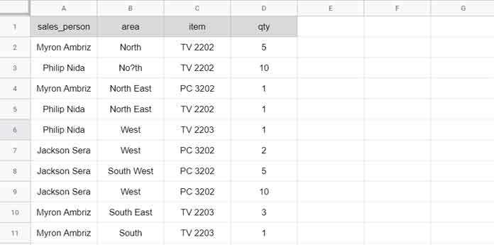
Example Scenario

I want the total quantity (Qty) of the item “TV.” There is no exact match for “TV” in column C. To partially match “TV” (e.g., “TV 2202,” “TV 2203”), we replace the wildcard asterisk with a combination of SEARCH and ISNUMBER in the formula:

=SUMPRODUCT(ISNUMBER(SEARCH("TV", C2:C11)), D2:D11)

Formula Explanation

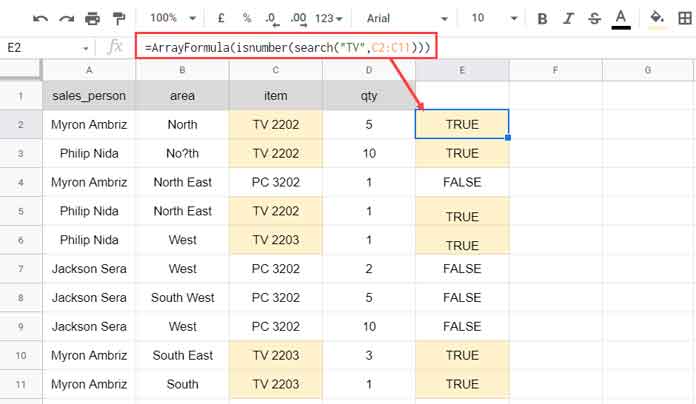
• ISNUMBER(SEARCH("TV", C2:C11)): The SEARCH function finds “TV” in the C2:C11 range and returns its position (a numeric value) for matching rows and a #VALUE! error for others. The ISNUMBER function converts numeric values to TRUE and errors to FALSE (an array of 1s and 0s).
• D2:D11: The array containing the quantities.
• SUMPRODUCT(...): Multiplies the arrays and sums the results, effectively summing quantities for rows where “TV” is found.

Note: If you use =ISNUMBER(SEARCH("TV", C2:C11)) outside SUMPRODUCT for testing, include ARRAYFORMULA for compatibility.

Using FIND with SUMPRODUCT in Google Sheets

If you need case sensitivity, replace SEARCH with FIND. The rest of the formula remains the same. For example:

=SUMPRODUCT(ISNUMBER(FIND("TV", C2:C11)), D2:D11)

Using REGEXMATCH Instead of Wildcards in SUMPRODUCT

The combination of SEARCH/FIND replicates the behavior of the asterisk wildcard for matching zero or more characters on either side. To handle other wildcard characters, such as:

• ?: Matches exactly one character.
• ~: Escapes * or ? to treat them as literal characters.

We can use REGEXMATCH with SUMPRODUCT. Let’s continue with the dataset in A1:D.

Examples

Note: The (?i) at the beginning of each pattern makes the match case-insensitive. To make it case-sensitive, remove (?i) from the regex pattern.

Simplification for Exact Matches

In some cases, REGEXMATCH is unnecessary. For example, the seventh formula can be replaced with:

=SUMPRODUCT(B2:B11="No?th", D2:D11)

Key Takeaways

Wildcards such as * and ? are not directly supported in SUMPRODUCT. However, you can replicate their functionality using combinations of SEARCH, FIND, or REGEXMATCH.

To enable flexible matching, pair ISNUMBER with SEARCH or FIND.

For advanced pattern matching, use REGEXMATCH, which also allows escaping special characters by using \.

That’s all about how to use wildcards in the SUMPRODUCT function in Google Sheets. Thanks for reading, and happy spreadsheeting!

Resources

• How to Use Date Differences as Criteria in SUMPRODUCT in Google Sheets
• Correctly Specifying Criteria in SUMPRODUCT in Google Sheets
• How to Do a Case-Sensitive SUMPRODUCT in Google Sheets
• How to Use OR Condition in SUMPRODUCT in Google Sheets
• How to Use SUMPRODUCT with Merged Cells in Google Sheets
• Wildcards in VLOOKUP Search Range in Google Sheets
• Filter Rows Based on Criteria List with Wildcards in Google Sheets