


")


")

")
")
 in Excel & Google Sheets")


How do you search up the first column of a table for a key instead of searching down using VLOOKUP? VLOOKUP from bottom to top is possible in Google Sheets—you just need to flip the table inside the VLOOKUP formula.
I know you can use LOOKUP or XLOOKUP instead of VLOOKUP to search up a column for a key and return a value from the row found. But that won’t satisfy a VLOOKUP user because of the flexibility that VLOOKUP offers.
At the end of this VLOOKUP tutorial, I’ll show you how to lookup the last occurrence of a key (which is equivalent to searching up) in a column using LOOKUP and XLOOKUP. But first, let’s look at the VLOOKUP formula.
How to VLOOKUP from Bottom to Top in Google Sheets
By default, VLOOKUP searches down the first column of a selected range. To make it search up, we need to flip the table used in the formula. Once we do this, VLOOKUP can return the first matching value from the bottom up.
If you’re familiar with flipping a table in Google Sheets, this won’t be difficult. The example below demonstrates the approach.
I have already covered how to flip a column in Google Sheets. If you want a detailed explanation, check out this tutorial: How to Flip a Column in Google Sheets – Finite and Infinite Columns.
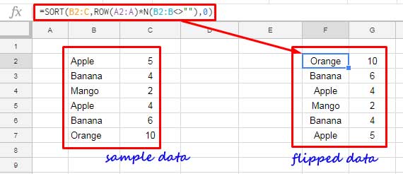
In the following example, my sample data is in the range B2:C. Here’s the formula to flip this table:
=SORT(B2:C, ROW(A2:A) * N(B2:B<>""), 0)This formula sorts the table in reverse row order while keeping blank rows at the bottom. The result can now be used as the lookup range in VLOOKUP.
How to Modify the Formula for Different Ranges
If your dataset is in a different range, update the formula accordingly. For example, if your data is in A1:E, use this:
SORT(A1:E, ROW(A1:A) * N(A1:A<>""), 0)Now that we have flipped the table, let’s apply VLOOKUP to search from bottom to top.
VLOOKUP from Bottom to Top in Google Sheets
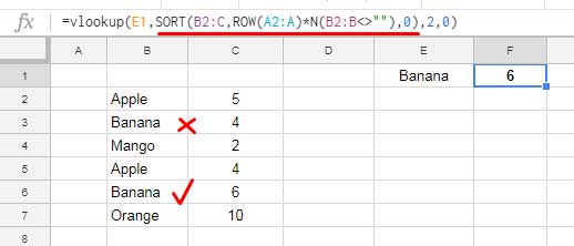
=VLOOKUP(E1, SORT(B2:C, ROW(A2:A) * N(B2:B<>""), 0), 2, 0)This formula searches for the key in E1 in the first column of the flipped range and returns the corresponding value from the second column.
Lookup the Last Occurrence Using the LOOKUP Function
As promised, here’s the LOOKUP version. This function naturally returns the last occurrence of a search key. However, it requires a sorted range. Since our data is unsorted, we need a workaround.
Instead of sorting the table, we’ll create a search range that contains 1 for matching rows and errors (#DIV/0!) elsewhere.
=ArrayFormula(1 / (B2:B = E1))Output:
{1; #DIV/0!; #DIV/0!; #DIV/0!; 1; #DIV/0!; ...}
This formula returns 1 in matching rows and #DIV/0! errors in others. Now, we use LOOKUP to find the last occurrence:
=LOOKUP(1, ArrayFormula(1 / (B2:B = E1)), C2:C)This formula effectively replaces VLOOKUP for bottom-to-top searches without flipping the table.
XLOOKUP Alternative
XLOOKUP natively supports bottom-to-top searches, regardless of whether the data is sorted.
For the same dataset, simply use:
=XLOOKUP(E1, B2:B, C2:C, , 0, -1)Breakdown of the Formula
E1: The search keyB2:B: The search rangeC2:C: The result range0: Exact match-1: Searches from bottom to top
However, VLOOKUP still has advantages in some cases. Let’s explore one such scenario.
VLOOKUP Multiple Search Keys from Bottom to Top
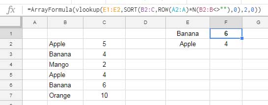
Assume you have multiple search keys in E1:E2. VLOOKUP and XLOOKUP both support this.
Using VLOOKUP:
=ArrayFormula(VLOOKUP(E1:E2, SORT(B2:C, ROW(A2:A) * N(B2:B<>""), 0), 2, 0))This formula searches E1:E2 in B2:C from bottom to top and returns the corresponding values.
Using XLOOKUP:
=ArrayFormula(XLOOKUP(E1:E2, B2:B, C2:C, , 0, -1))However, if you have a third column, i.e. D2:D and want the result from both C2:C and D2:D, XLOOKUP won’t work with multiple search keys as shown above—but VLOOKUP will.
=ArrayFormula(VLOOKUP(E1:E2, SORT(B2:D, ROW(A2:A)*N(B2:B<>""), 0), {2, 3}, 0))That said, XLOOKUP remains simpler and can look up to the left, which VLOOKUP cannot do without a workaround, such as rearranging the column order.