")
")


")


")

")
")
 in Excel & Google Sheets")


Google Sheets doesn’t natively support showing group totals when you manually group rows using View > Group. But with a dynamic formula setup, you can still display totals for collapsed groups and subgroups in Google Sheets. This works well when your data is organized hierarchically.
Before we dive into the steps, here’s a sample Google Sheet with the dataset, grouping structure, helper table, and formulas:
Open Sample Sheet – Explore the setup to better understand how this works.
Now, the dataset:
Let’s first see a sample data:
Sample Data
| Sr. No. | Item | Sales | Group Total |
| 1 | Electronics | ||
| 1.1 | Phones | ||
| iPhone | 800 | ||
| Galaxy | 750 | ||
| Pixel | 620 | ||
| 1.2 | TVs | ||
| Sony Bravia | 900 | ||
| LG OLED | 870 | ||
| 2 | Furniture | ||
| 2.1 | Chairs | ||
| Office Chair | 150 | ||
| Gaming Chair | 230 | ||
| 2.2 | Tables | ||
| Coffee Table | 300 | ||
| Dining Table | 500 | ||
| Total | 5120 |
The structure — using labels like “1”, “1.1”, “2”, etc. — visually defines the hierarchy of categories and subcategories, which helps when applying grouping.
How to Apply Grouping in Google Sheets
- Select rows with items under each subcategory (e.g., the rows with iPhone, Galaxy, and Pixel).
- Go to View > Group rows — this allows you to collapse the subcategory.
- Repeat for all subcategories.
- For each main category, select all the relevant subcategory rows (e.g., rows 3 to 9 for Electronics).
- Again, go to View > Group rows to collapse the main category.
- Repeat for all main categories.
With this setup, let’s move to the core logic behind how to display totals for collapsed groups and subgroups in Google Sheets.
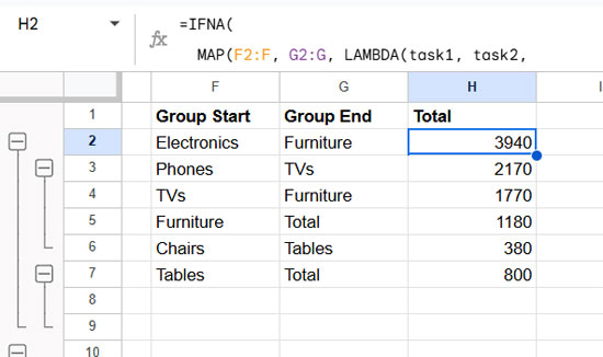
Step 1: Create a Helper Table with Group Start and End Points
In columns F and G, prepare a helper table like this:
| Group Start | Group End |
| Electronics | Furniture |
| Phones | TVs |
| TVs | Furniture |
| Furniture | Total |
| Chairs | Tables |
| Tables | Total |
This table outlines where each group or subgroup starts and ends.
Tip: If you don’t have a Total row at the bottom, replace it with a placeholder like an underscore _ in both your dataset and this helper table.
Step 2: Formula to Calculate Totals for Groups/Subgroups
In cell H2, enter the formula:
=IFNA(
  MAP(F2:F, G2:G, LAMBDA(task1, task2,
     SUM(XLOOKUP(task1, B2:B, C2:C):OFFSET(XLOOKUP(task2, B2:B, C2:C), -1, 0)))
  )
)
What This Formula Does:
- XLOOKUP(start, B2:B, C2:C) returns the first cell in the sales column for the group start.
- XLOOKUP(end, B2:B, C2:C) returns the first cell for the group end.
- OFFSET(…, -1, 0) moves one row up from the end point (to exclude the group label row).
- Using the colon
:with these two points defines a range. - SUM(…) totals the values within that range.
- MAP applies this logic row by row for every pair in your helper table (F2:F and G2:G).
As a result, column H will display the total sales for each group or subgroup.
If you’d like to dive deeper into how this kind of formula logic works, check out:
- Slicing Data with XLOOKUP in Google Sheets
- Count Rows and Entries Between Two Values in Google Sheets
Step 3: Display Totals for Collapsed Groups and Subgroups
Now that you have group totals in column H, let’s show them conditionally — only when their corresponding group is collapsed.
In cell D2, enter the following formula:
=ArrayFormula(
  LET(
     hidden, CHOOSEROWS(MAP(B2:B, LAMBDA(row, SUBTOTAL(103, row))), SEQUENCE(ROWS(B2:B)-1, 1, 2)),
     total, CHOOSEROWS(XLOOKUP(B2:B, F2:F, H2:H), SEQUENCE(ROWS(B2:B)-1, 1, 1)), IFNA(IF(hidden=0, total,))
  )
)
Breakdown of the Formula:
- SUBTOTAL(103, row) checks if the row is visible (
1) or hidden (0). - MAP + CHOOSEROWS(…, SEQUENCE(…)) skips the first row to align visibility flags correctly with your data rows.
- XLOOKUP(B2:B, F2:F, H2:H) fetches the group total for each label in your main column.
- IF(hidden = 0, total, ) — if the group row is hidden (i.e., collapsed), show the total.
So when a group is collapsed (the “-” turns to “+”), this formula will show the group’s total in column D, right at the group header row.
Conclusion
This technique works best when your data is organized with a clear hierarchy and proper row grouping. It provides a smart workaround to display totals for collapsed groups and subgroups in Google Sheets, even though the feature isn’t supported natively.
The best part is that the formulas are dynamic — you don’t need to modify them each time you add or remove groups or subgroups. The only thing you’ll need to update is the Group Start and Group End helper table to reflect your new structure.
Both formulas in cells D2 and H2 automatically cover the full dataset, so once set up, there’s no need to edit them manually.
Thanks for posting this information.
I’m having a hard time duplicating this functionality with grouped/ungrouped columns.
Is that functionality possible?
Hi, Miles Garrett,
As far as I know, it’s not possible to replicate the same thing with columns.