Before we dive into the SUMIF to sum by current work week formula in Google Sheets, it’s important to understand what a work week means in this context.
A work week typically consists of 5 days, spanning from Monday to Friday. However, depending on your region or organization, it can also run from Monday to Saturday or even Sunday to Thursday. We can handle these variations effectively using the WORKDAY function within the SUMIF criteria.
You can use the following formula to sum values for the current work week in Google Sheets:
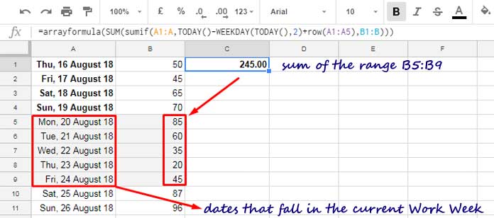
=ARRAYFORMULA(SUM(SUMIF(A1:A, TODAY()-WEEKDAY(TODAY(), 2)+ROW(A1:A5), B1:B)))This formula sums the range B1:B corresponding to the dates in column A that fall within the current work week, typically from Monday to Friday.
In the example below, I’ll also explain how to modify this formula to adjust the work week to match your specific needs.
Example of SUMIF to Sum by Current Work Week
Assume you have material purchase dates in column A and quantities in column B. You want to total the quantity received during the current work week, from Monday to Friday.
You can use the formula mentioned earlier in C1.

The formula dynamically adjusts to the current work week, so you don’t need to update it manually each week.
Adjusting the Work Week in the Formula
To customize the work week, modify the WEEKDAY(TODAY(), 2) part of the formula as follows:
WEEKDAY(TODAY(), 2)– For a work week from Monday to Friday.- WEEKDAY(TODAY(), 1) – For a work week from Sunday to Thursday.
If you want to include Monday to Saturday (6 working days), use the corresponding WEEKDAY formula and adjust the ROW(A1:A5) part to ROW(A1:A6).
SUMIF to Sum by Current Work Week: Formula Breakdown
Let’s break down the SUMIF to sum by current work week formula:
SUMIF(range, criterion, [sum_range])Here’s how the formula components are defined:
- range:
A1:A, which is the date column. - criterion:
TODAY()-WEEKDAY(TODAY(), 2)+ROW(A1:A5), which generates dates for the current work week. - sum_range:
B1:B, which is the column containing the values to sum.
In the criterion, TODAY()-WEEKDAY(TODAY(), 2) calculates the start of the week (Monday). The ROW function, such as ROW(A1:A5), adds a sequence of days to generate dates for the week.
The SUMIF formula totals column B for rows in column A that match the criterion. This calculates the total values corresponding to the current work week.
The SUM function then aggregates these values into a single total.
We used ARRAYFORMULA for two reasons:
- To handle multiple conditions, as SUMIF requires array support.
- To create the criterion using an array of dates.
Additional Tip
You can generate dates for the current work week in different ways. In the formula above, we used the following approach:
TODAY()-WEEKDAY(TODAY(), 2)+ROW(A1:A5)Here, ROW(A1:A5) generates a sequence of numbers. If you prefer, you can replace it with SEQUENCE(5). For a 6-day work week, use ROW(A1:A6) or replace it with SEQUENCE(6).
Alternatively, you can specify the criteria using this formula:
SEQUENCE(5, 1, TODAY()-WEEKDAY(TODAY(), 2))This SEQUENCE function generates dates in 5 rows and 1 column, starting from TODAY()-WEEKDAY(TODAY(), 2).
If your work week has 6 days, change 5 to 6 in the formula. To start the week from Sunday, replace WEEKDAY(TODAY(), 2) with WEEKDAY(TODAY(), 1).


