When using the QUERY function with a PIVOT clause in Google Sheets, you might notice that pivot headers are sorted in ascending order by default. But what if you need them sorted in descending order? Unfortunately, the QUERY function doesn’t offer a direct option for this. However, with a clever workaround, you can achieve this sorting seamlessly.

In this tutorial, let’s explore step-by-step how to sort QUERY pivot headers in descending order. Whether you’re working with numerical, text, or date headers, this method will help you organize your data exactly the way you need.

Logic

The logic behind sorting QUERY pivot headers in descending order is simple: swap the SELECT and GROUP BY column with the PIVOT column.

Note: The PIVOT clause in a QUERY can be used with or without the GROUP BY clause. When the GROUP BY clause is omitted, the output will typically consist of headers in one row and totals in another row. However, QUERY Pivot usually involves a GROUP BY clause, as it enables more detailed grouping and analysis. Our examples are based on this common use case.

Sample Data

The sample data is as follows:

Columns A, B, and C contain the purchase date, item, and amount, respectively. The range is A1:C, where A1:C1 contains the headers.

We will use this data to create three pivot tables, each with text, number, and month names as headers sorted in descending order. For the first two, the headers will be sorted Z-A, while for the third, the month name headers will be sorted in descending chronological order.

Sort QUERY Text Pivot Headers in Descending Order

In the above data, assume you want to find the date-wise purchase amount for each item. You want the dates in rows and items in columns.

Typically, you would group the date column and pivot the item column. This gives the desired result, but it sorts the items in ascending order.

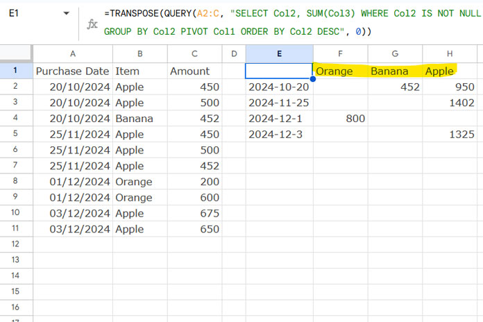
To sort the QUERY pivot headers (items) in descending order, you need to swap the SELECT column and the PIVOT column. The items will appear in rows and dates in columns. You can then sort the items in descending order using the ORDER BY clause and transpose the result:

=TRANSPOSE(QUERY(A2:C, "SELECT Col2, SUM(Col3) WHERE Col2 IS NOT NULL GROUP BY Col2 PIVOT Col1 ORDER BY Col2 DESC", 0))

Sort QUERY Numeric Pivot Headers in Descending Order

The same approach works for numeric pivot headers. For example, to find the month-wise sales amount of items, you may want the item names in rows and the month numbers in headers.

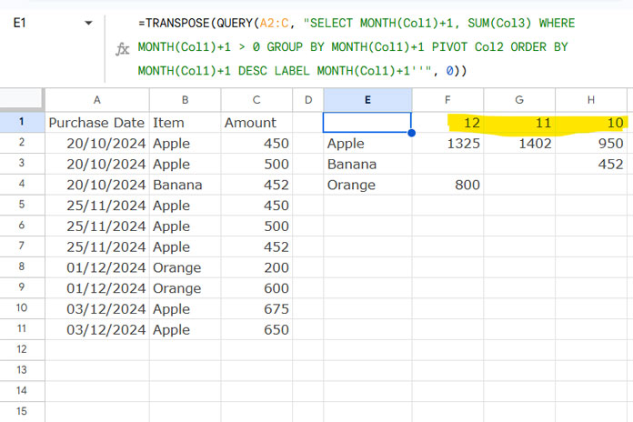
Group by the month number, pivot the items, and transpose the result:

=TRANSPOSE(QUERY(A2:C, "SELECT MONTH(Col1)+1, SUM(Col3) WHERE MONTH(Col1)+1 > 0 GROUP BY MONTH(Col1)+1 PIVOT Col2 ORDER BY MONTH(Col1)+1 DESC LABEL MONTH(Col1)+1''", 0))

We use MONTH(Col1)+1 instead of just MONTH(Col1) to adjust the month numbers. The default month numbering in QUERY starts from 0 (for January) to 11 (for December), but by adding 1, we convert the month range to 1 to 12. Additionally, we use the LABEL clause to remove the header corresponding to the month number. Without this, the first cell of the pivot table might display something like sum(month()1()), which we want to avoid.

Sort Month Names in QUERY Pivot Headers Chronologically

Now let’s explore the most interesting part: sorting QUERY pivot headers with month names in descending chronological order.

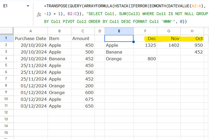
The logic is similar to the previous examples, but the data preparation requires extra steps. Month names default to alphabetical sorting. To overcome this, transform the dates into month start dates and format them as month text. This ensures the pivot headers retain their chronological order while displaying as month names.

Here’s the formula:

=TRANSPOSE(QUERY(ARRAYFORMULA(HSTACK(IFERROR(EOMONTH(DATEVALUE(A2:A), -1) + 1), B2:C)), "SELECT Col1, SUM(Col3) WHERE Col1 IS NOT NULL GROUP BY Col1 PIVOT Col2 ORDER BY Col1 DESC FORMAT Col1 'MMM'", 0))

Explanation of the Data Preparation:

The data part of the formula is ARRAYFORMULA(HSTACK(IFERROR(EOMONTH(DATEVALUE(A2:A), -1) + 1), B2:C)). Here’s a breakdown of each function:

1. DATEVALUE(A2:A): Converts dates in A2:A to date values, returning errors for non-date cells.
2. EOMONTH(..., -1) + 1: Returns the start date of each month, leaving errors untouched. Blank cells are treated as serial number 0, corresponding to 30/12/1899. The DATEVALUE in the first step prevents this from happening by ensuring only valid date values are processed.
3. IFERROR(...): Replaces errors with blanks.
4. HSTACK(..., B2:C): Horizontally stacks the processed dates with columns B and C.

The QUERY function uses this processed data to sort the month start dates in descending order while formatting them as month names with the FORMAT clause. Transposing the result restores the desired layout.

Conclusion

This tutorial demonstrated three examples to sort QUERY pivot headers in descending order in Google Sheets:

• Sorting text headers Z-A
• Sorting numeric headers Z-A
• Sorting month names in descending chronological order

These methods should help you tackle any challenges with sorting QUERY pivot headers effectively. If you have questions, feel free to ask in the comments.

Resources

• Month Name as the Criterion in QUERY Date Column
• Using QUERY Function Similar to Pivot Table in Google Sheets
• How to Format QUERY Pivot Header Row in Google Sheets
• How to Pivot Multiple Columns in QUERY in Google Sheets
• Replace Blank Cells with 0 in QUERY Pivot in Google Sheets
• How to Retain All Column Labels in QUERY Pivot in Google Sheets
• Google Sheets QUERY: Convert Month Number to Month Name