You can sort alphanumeric values directly within the original range or use a formula to sort them into a new range in Google Sheets. The former method requires a helper formula.

There are many scenarios where a spreadsheet may contain alphanumeric values in a column, such as product codes, invoice numbers, student or employee codes, and vehicle license plates.

Here’s how to sort alphanumeric values properly in Google Sheets.

Sort Alphanumeric Values Using a Formula in Google Sheets

In the following example, employee codes are in column A, and employee names are in column B.

Use the following formula in cell D2 to sort the data by the alphanumeric values in column A:

=SORT(A2:B, REGEXEXTRACT(A2:A,"\D+"), TRUE, VALUE(REGEXEXTRACT(A2:A,"\d+")), TRUE)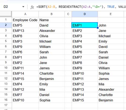

Formula Explanation

The formula is based on the SORT function. Its syntax is:

SORT(range, sort_column, is_ascending, [sort_column2, …], [is_ascending2, …])

Here’s how the components work:

• range:
  A2:B specifies the range to sort.
• sort_column:
  REGEXEXTRACT(A2:A, "\D+") extracts the first sequence of non-digit characters (e.g., letters or special characters) from the alphanumeric values in column A.
• is_ascending:
  TRUE sorts the range by the extracted text in ascending order.
• sort_column2:
  VALUE(REGEXEXTRACT(A2:A, "\d+")) extracts the first sequence of digits from column A and converts them into numeric values.
• is_ascending2:
  TRUE sorts the range by the numeric part in ascending order.

In summary, the formula extracts text and numeric components separately and uses them as sort columns to sort alphanumeric values in Google Sheets.

Sort Alphanumeric Values Using the Sort Menu in Google Sheets

One limitation of sorting with a formula is that you can’t directly edit the sorted output. Changes must be made in the source data range. If you want to sort alphanumeric values directly in the original range, you can use the Sort Menu with the help of a helper column.

Steps:

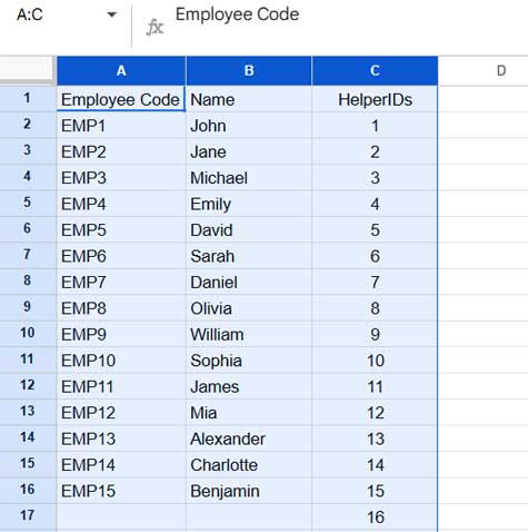
Using the same sample data, insert the following formula in the first row of an empty column next to the data. For this example, insert it in C1:

=ArrayFormula(
   LET(
      alphaN, A2:A, 
      textE, REGEXEXTRACT(alphaN,"\D+"), 
      numberE, VALUE(REGEXEXTRACT(alphaN,"\d+")), 
      seqR, SEQUENCE(ROWS(alphaN)), 
      srt, CHOOSECOLS(SORT(HSTACK(seqR, alphaN), textE, TRUE, numberE, TRUE), 1), 
      VSTACK("HelperIDs", XMATCH(seqR, srt))
   )
)

After inserting the formula, follow these steps:

1. Select the range A1:C.
2. Go to Data > Sort range > Advanced range sorting options.
3. Check Data has a header row.
4. Choose “HelperIDs” under Sort by.
5. Click Sort.

This will sort the data by the employee codes in column A in the correct alphanumeric order.

Understanding the Helper Column Formula

1. textE:
   • REGEXEXTRACT(A2:A, "\D+"): Extracts the first sequence of non-digit characters.
2. numberE:
   • VALUE(REGEXEXTRACT(A2:A, "\d+")): Extracts the first sequence of digits and converts them to numbers.
3. seqR:
   • SEQUENCE(ROWS(A2:A)): Generates sequence numbers for the rows in the range.
4. srt:
   • HSTACK(seqR, A2:A): Combines the sequence numbers with the original range.
   • SORT(..., textE, TRUE, numberE, TRUE): Sorts the alphanumeric values based on textE and numberE.
   • CHOOSECOLS(..., 1): Extracts the sorted sequence numbers.
5. Final Expression:
   • VSTACK("HelperIDs", XMATCH(seqR, srt)): Stacks the header “HelperIDs” and the relative positions of the sequence numbers from the sorted data.

The sorted alphanumeric values are displayed based on the helper column.

Additional Resources

• Sort Text-Formatted or Multi-Level Numbers in Google Sheets
• Sort by Custom Order in Google Sheets [How to Guide]
• Formula for Sorting by Month Name in Google Sheets
• Dynamic Sort Column and Sort Order in Google Sheets
• Fix Array Formula Messing Up When Sorting in Google Sheets