


")


")

")
")
 in Excel & Google Sheets")


Before highlighting the smallest N values in a row—or in each row—you should decide how to handle duplicates and ties at the Nth position. The table below outlines the options:
| Value | Strictly Lowest N | Lowest N + Ties of Nth | Distinct Lowest N |
| 1 | ✅ | ✅ | ✅ |
| 1 | ✅ | ✅ | |
| 2 | ✅ | ✅ | ✅ |
| 2 | ✅ | ||
| 3 | ✅ |
Here are the custom formula rules to highlight the smallest N values in a row or each row in Google Sheets.
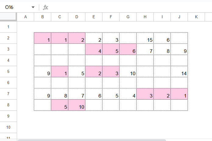
Rule 1: Strictly Lowest N in a Row or Each Row
=AND(LEN(B2), XMATCH(CELL("address", B2), SORTN(TOCOL(ADDRESS(ROW($B2:$J2), COLUMN($B2:$J2))), 3, 0, TOCOL($B2:$J2), TRUE)))This formula highlights the smallest N values in each row, excluding ties at the Nth position.
Replace $B2:$J2 with your desired row range, B2 with the first cell in the range, and 3 with your preferred N value.
You can apply this to a single row (e.g., $B2:$J2) or multiple rows (e.g., $B2:$J8) without modifying the formula. Just update the “Apply to range” field accordingly in the Conditional Formatting Rules panel.
Example:
- Select the range
B2:J8 - Go to Format > Conditional formatting
- Under Format rules, select Custom formula is, and paste the formula
- Choose a formatting style and click Done
How it works:
TOCOL(ADDRESS(ROW($B2:$J2), COLUMN($B2:$J2)))returns the cell addresses of each value in the row.SORTN(..., 3, 0, TOCOL($B2:$J2), TRUE)gives the addresses of the lowest 3 values.XMATCHchecks if the current cell’s address is among them.ANDensures the cell isn’t blank and that it’s one of the lowest 3.
This works row-by-row because the formula uses absolute column references and relative row references.
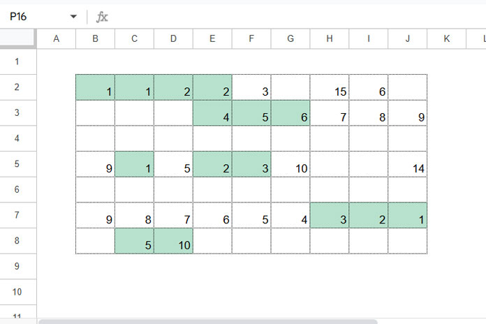
Rule 2: Lowest N + Ties of Nth in a Row or Each Row
=RANK(B2, $B2:$J2, TRUE)<=3Use this to highlight the lowest 3 values plus any values tied at the 3rd lowest spot.
Update $B2:$J2 with the first row of your data and B2 with the first cell in that row.
Follow the same steps as in Rule 1 to apply this rule.
How it works:
- The
RANKfunction assigns the smallest value a rank of 1, the next smallest 2, and so on. - Tied values share the same rank, and subsequent ranks skip accordingly.
- All cells with rank ≤3 get highlighted.
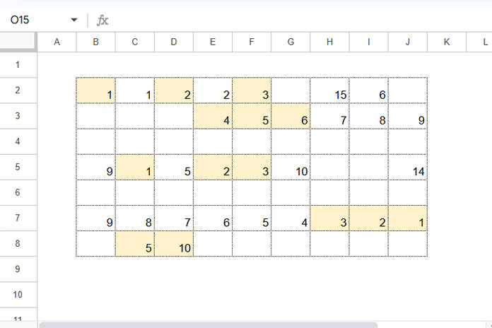
Rule 3: Distinct Lowest N in a Row or Each Row
=AND(XMATCH(B2, SORTN(TOCOL($B2:$J2), 3, 2, 1, TRUE)), COUNTIF($B2:B2, B2)=1)Use this to highlight the smallest 3 distinct values in each row—ignoring duplicates.
Replace $B2:$J2 with the first row in your data, B2 with the first cell, and $B2:B2 with a corresponding range.
How it works:
SORTN(TOCOL($B2:$J2), 3, 2, 1, TRUE)returns the smallest 3 unique values.XMATCH(B2, ...)checks if the current cell is among them.COUNTIF($B2:B2, B2)=1ensures only the first occurrence of each value is considered.ANDreturns TRUE only if both conditions are met.
Resources
- Highlight the Smallest N Values in a Column in Google Sheets
- Average of Smallest N Values in Google Sheets (Zero and Non-Zero)
- Lookup the Smallest Value in a 2D Array in Google Sheets
- Finding Max and Min Values in GoogleFinance Historical Data in Sheets
- How to Highlight the Min Value in Each Group in Google Sheets
- Find Minimum Value and Return Value from Another Column – Google Sheets
- Find the Running Minimum Value in Google Sheets
This tutorial has shown multiple ways for how to highlight the smallest N values in each row in Google Sheets. Depending on your preference—strictly N, tied Nth, or distinct—you can choose the right rule for your spreadsheet.