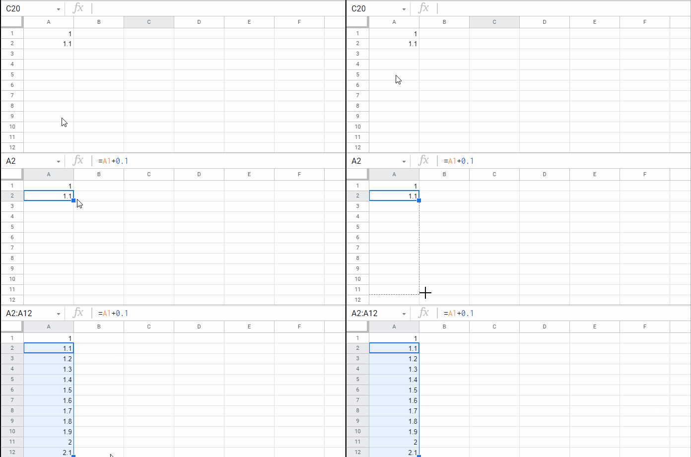
How to Create a Sequence of Decimals in Google Sheets

If you ever needed a smooth list like 1, 1.1, 1.2, ... 1.9, 2, 2.1, 2.2, ..., 2.9, 3 in Google Sheets, you’re in the right place. Whether you’re working with decimal-based values or just need more precise row numbering, Google Sheets offers a few simple ways to create a sequence of decimals.

In this post, I’ll walk you through three easy methods:

Using the fill handle (good for quick lists)
Writing a formula and dragging it down
And my personal favorite — using the SEQUENCE function for dynamic, no-fuss results

Table of Contents

1. Create a Sequence of Decimals by Dragging Adjacent Cells

This is probably the most intuitive method if you’re just getting started.

Steps:

Type 1 in cell A1
Type 1.1 in A2
Select both cells (A1:A2), and drag the fill handle downward

Note: The fill handle is that small circle at the bottom-right corner of your selection. (It used to be a square in earlier versions of Google Sheets.) Just drag it down to autofill the pattern.

Google Sheets is smart enough to pick up the decimal pattern and continue it — you’ll see 1.2, 1.3, and so on.

Want something like `0.25, 0.5, 0.75…`?

No problem. Just:

Type 0.25 in A1
Type 0.5 in A2
Select both, then drag down

Done!

2. Create a Sequence of Decimals Using a Simple Formula

If you want a bit more control (and maybe prefer formulas), this method is perfect.

Here’s how:

Enter 1 in A1
In A2, type:
=A1 + 0.1
Drag the formula in A2 down the column

Creating a decimal sequence in Google Sheets by dragging a formula down (GIF)

This will build the same decimal sequence. And just like before, you can adjust the step — for example, use =A1+0.25 if you want to increment by 0.25.

Why use this?

While it takes slightly longer than the fill handle, you get more consistency and control. Plus, it’s easier to tweak later if your step size or starting value changes.

3. Use the SEQUENCE Function (The Smartest Way)

If you’re into neat, scalable solutions, this one’s for you. The SEQUENCE function can generate a full column of decimals in one go — no dragging or manual setup.

The formula:

=SEQUENCE(20, 1, 1, 0.1)

Let’s break that down:

20 → the number of rows (i.e., how many decimal numbers you want)
1 → number of columns (we’re making a vertical list)
1 → start value
0.1 → step (each number increases by 0.1)

It will return:

Want different step sizes?

Try this one:

=SEQUENCE(20, 1, 0.25, 0.25)

That will generate:

Super clean. Super flexible.

So, Which Method Should You Use?

All three methods work — but they each serve different needs:

Quick drag with the fill handle is great for short, one-off lists
Formula-based fill gives you slightly more control, and works well for manual setups
SEQUENCE is the clear winner for anything dynamic, automated, or long-term

Also, both the drag-fill method and the fill-down formula can break if you insert or delete rows within the range. SEQUENCE doesn’t care — it just keeps generating values without getting disrupted. So for anything dynamic or long-term, SEQUENCE is definitely the way to go.

Wait — What If You Meant 1, 1.1, 1.2, 2, 2.1…?

If you’re looking to create a structured format like:

That’s actually a different type of decimal sequence — more like an outline-style or hierarchical row numbering.

I’ve written a separate guide just for that:

👉 How to Number Rows as 1, 1.1, 1.2 in Google Sheets (Hierarchical Format)

Check that out if that’s what you were after.

Conclusion

Creating a sequence of decimals in Google Sheets is easy once you know your options. Whether you’re building time intervals, score progressions, or simply need decimal-based IDs — these techniques have you covered.

For the cleanest, most flexible option, I definitely recommend using the SEQUENCE function. It saves time and keeps your data dynamic.