


Here is a link building technique in Google Sheets. You can search value and hyperlink cell that found (in a list). The search key and lookup list can be in same sheet tab or two different sheet tabs.
Here is the approach that I am following in this tutorial. I have a Google Sheets file with two tabs – Sheet1 and Sheet2. In that file Sheet1!A1:A contains a list of names.
In Sheet2!A1 I have a name. I want to search that name in Sheet1!A1
How to Search Value and Hyperlink Cell Found
To save time, I am going to import a table in Sheet1. You can follow me to import an external list for testing my formulas below.
Just use this formula in Sheet1!A1 in your Google Sheets file. The sheet should be blank.
=IMPORTHTML("https://en.wikipedia.org/wiki/List_of_states_and_territories_of_the_United_States","table",1)The above IMPORTHTML formula will populate an entire table contains the names of states and territories of the United States (see the source Wiki page).
For the example purpose, I mean to search value and Hyperlink cell found, we only need a one column list. So, modify the formula as below. I have used the function Index to limit the columns to 1.
=Index(IMPORTHTML("https://en.wikipedia.org/wiki/List_of_states_and_territories_of_the_United_States","table",1),0,1)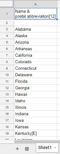
Now in
Steps to Hyperlink a Value to a Cell in a List in Google Sheets
Here are the steps involved. In Sheet1!B1 enter this ArrayFormula.
=ArrayFormula(if(len(A1:A),"URL"&row(A1:A),))Right click on the cell A1 in Sheet1 and select “Get
At the last part of the
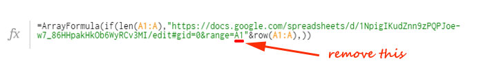
See my formula. The URL will be different for you.
=ArrayFormula(if(len(A1:A),"https://docs.google.com/spreadsheets/d/1NpigIKudZnn9zPQPJoe-w7_86HHpakHkOb6WyRCv3MI/edit#gid=0&range=A"&row(A1:A),))The above formula generates an array of URLs connected to the values in column A.
Now see how to search value and Hyperlink to the cell found in Google Sheets. To do that go to Sheet2!B1. In that sheet in cell A1, I have the key “Hawaii”.
I am searching this value in Sheet1, column 1 and link to the cell in Sheet1.
Use this formula in Sheet2!B1. It searches the value “Hawaii” in Sheet1, column 1 and returns the URL from column 2.
=vlookup(A1,Sheet1!A1:B,2,0)That means the above formula will return the URL of the cell Sheet1!A13. Clicking on that URL will take you to the relevant cell in Sheet1. But what we want is Hyperlink.
Syntax:
HYPERLINK(URL, [link_label])In this replace the URL with the above Vlookup based formula and link_label with A1.
So the final formula in cell B1 in Sheet2 will be as follows.
=hyperlink(vlookup(A1,Sheet1!A1:B,2,0),A1)The above is the formula to search
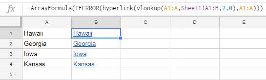
If you want to search multiple values in a list and bulk hyperlink, the formula would be as follows.
=ArrayFormula(IFERROR(hyperlink(vlookup(A1:A,Sheet1!A1:B,2,0),A1:A)))Output:
Conclusion
I know it’s not a common task to search value and Hyperlink to the cell found. But I can see many users use this in Excel. The approach is entirely different in Excel and Sheets.
If you are one who switched from Excel then you may find the above hyperlinking tips useful.
Hi Prashanth, perfect, it was very fast. Thanks a lot for your help. It works very well. Regards.
Hi, It works well!
Is it possible to hyperlink matched value by the functions INDEX/MATCH instead of the VLOOKUP?
Thanks.
Yes! I will update you with a tutorial soon.
Hi, Roman,
It’s ready now!
Hyperlink to Index-Match Output in Google Sheets.
Cheers!