The INDIRECT function is essential when creating a conditional formatting rule that references cells across different sheet tabs in Google Sheets.
In other words, you cannot directly refer to a cell in another sheet within the custom formula field for conditional formatting.
For example, let’s say you have two sheets: one named “Find Group” and the other “Student Group.”
If your active sheet is “Find Group,” you would normally refer to cell A1 in “Student Group” like this:
='Student Group'!$A$1However, you cannot use this reference directly in the custom formula field for conditional formatting. Instead, you need to use the INDIRECT function, like this:
=INDIRECT("Student Group!A1")Let me give you a real-life example.
Example
I am confident that you will appreciate the following example, where I will use the INDIRECT function in conditional formatting.
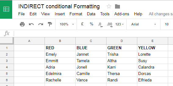
I have a dataset containing student names in a sheet named “Student Group,” categorized under different groups. There are four groups named RED, BLUE, GREEN, and YELLOW in cells B1:E1. Under each header, the student names belonging to those groups are listed.

Assume these students have participated in various competitions during a school annual day event.
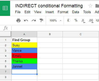
I have the names of the winners in another sheet in column A, without the associated group names. In that sheet, named “Find Group,” I want to highlight the cell with the group color when I enter the name of any winner from any group.

I will explain how we can achieve this, and along the way, you will also learn the role and use of the INDIRECT function in conditional formatting.
INDIRECT in Custom Formula Rules for Conditional Formatting
Let’s review the conditional formatting rules for the example above.
We will apply conditional formatting to the range A2:A in the “Find Group” sheet (refer to screenshot #2). However, the reference data is located in the range B2:E in the “Student Group” sheet (refer to screenshot #1).
Since there are four groups in four columns, we need four custom formulas to achieve this.
=XMATCH(A2, INDIRECT("'Student Group'!B:B")) // red
=XMATCH(A2, INDIRECT("'Student Group'!C:C")) // blue
=XMATCH(A2, INDIRECT("'Student Group'!D:D")) // yellow
=XMATCH(A2, INDIRECT("'Student Group'!E:E")) // green
These XMATCH formulas check if the name in cell A2 matches any names in columns B, C, D, and E of the “Student Group” sheet and return either a number or #N/A.
Wherever the formulas return a number, the corresponding cells in column A of the “Find Group” sheet will be highlighted.
Using INDIRECT Formulas for Conditional Formatting
Here’s how to apply the above rules and highlight student names based on their group.
Ensure that cell A2 is the active cell in the “Find Group” sheet. Then, click Format > Conditional formatting.
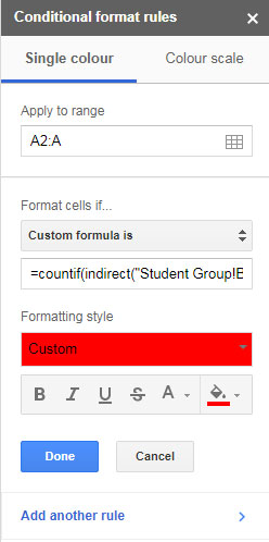
Under “Apply to range,” enter A2:A or A2:A100 (depending on your preferred range).
In the “Format cells if…” drop-down menu, select Custom formula is and copy-paste the first formula.
Under “Formatting style,” select the color Red.

Click “Add another rule,” then copy and paste the second formula. Change the color to Blue. Repeat this process for the other two formulas, setting their corresponding colors.
To test if all the formulas work as expected, enter the name of a student from any group in the A2:A range of the “Find Group” sheet. The cell should be highlighted according to the student’s group color.
Note: Avoid copying and pasting names, as this may remove the conditional formatting rules you’ve set.
Here is my sample Google Sheets file.
Resources
Here are two more tutorials where I have used the INDIRECT function in conditional formatting in Google Sheets:


I am trying to shade some cells based on the numerical value in another cell.
I have have tried many options, but it does not seem to work in Google Sheets.
E.g., in cell A1 I put the value 6. So then I want this to shade the cell range A6:C6.
…how simple is that, but I cannot achieve it.
I have tried using the Indirect and Index functions in the conditional formatting, but it doesn’t work.
Any ideas, please?
Hi, Giles,
This formula will highlight A1:C1 if A1 is 1, A2:C2 if A1 is 2, and so on.
=INDEX(LET(control_cell,A1,range,INDIRECT("A"&$A$1&":C"&$A$1),
MATCH(CELL("address",control_cell),ADDRESS(ROW(range),COLUMN(range)),0))
)
Apply to range: A1:C1000.
Goal:- Have the cell change color once the original number is replaced with a new number.
Thanks for any potential help!
Hi, Jack Christmann,
You may require Apps Script to do that. Sorry, I am not familiar with that.
I tried using your formula, but it does not apply the formatting correctly. Instead of formatting only the cells in the range that match the criteria, it formats the entire range if one cell matches. How do I get it to stop doing that?
Did you check my example sheet?
I can use a named range to refer to a cell in another sheet, right? I have tried this in the following formula
=IF($A80,IF(AND(($M8+Last_contact_followup<=TODAY()),S8"Won"),TRUE,FALSE),"")and I get an error message if I put this formula into Conditional formatting / Custom formula in a Google Sheet.The error comes from the named range “Last_contact_followup” and I have no idea why? This works in Excel but not in Google Sheets. Where do I get wrong?
Hi, Thomas,
I don’t know what you are trying to achieve. So it’s tough for me to correct the formula.
I am sure that the formula is not coded correctly. For example, take a look at the AND use. I guess there is a small typo in your formula. It must be as below.
=AND($M8+Last_contact_followup<=TODAY(),S8="Won")This part will work correctly. It would return TRUE or FALSE. But in conditional formatting use Indirect with the named ranges as below.
=AND($M8+indirect("Last_contact_followup")<=TODAY(),S8="Won")It will highlight the "Apply to range" cell (see the conditional formatting panel) to your set color if the output is TRUE, else blank. I don't know why you are using the IF statement. It may not be required in conditional formatting.
Best,