


To know how to keep or retain all the column labels in a Query Pivot in Google Sheets, you must know the reason for the missing columns.
We may get data in multiple rows (not necessarily) when using the Group By clause together with the Pivot clause in Query.
I mean to say, we will get a table where each cell contains the aggregation result for the relevant row (Group By) and column (Pivot).
When you use the Where clause to filter out some of the rows in the grouping, the relevant column(s) may become blank and subsequently disappear from the output.
This post explains how to retain all column labels in Query Pivot in Google Sheets.
For example, running the following QUERY in cell G1 on the table range C1:E will return the response shown in G1:I3.
=query({C1:E},"Select Col1, sum(Col3) where Col1 is not null group by Col1 pivot Col2")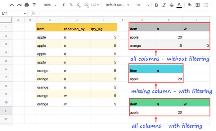
See what happens in G6:H7 when we filter out “orange” by running the following Query in G6.
=query(C1:E,"Select C, sum(E) where C='apple' group by C pivot D")One Pivot column label is missing!
How to retain all column labels as per G10:I11 in Query Pivot in Google Sheets?
We will see to that with two examples below.
Retaining All Column Labels in Query Pivot – Criterion in Select Clause Column
If you check the three Query responses in columns G1:I above, you will get the logic to keep all the columns in the Pivot table.
What is that?
To retain all column labels in Pivot, nest two Query formulas.
We will apply the criterion in the outer Query.
I have the following formula in G10, where you can see the highlighted ‘moved’ criteria.
=query(query(C1:E,"Select C, sum(E) where C is not null group by C pivot D"),"Select * where Col1='apple'")The above logic applies only when you filter the column specified in the Select clause.
It’s that simple to retain all column labels in Query Pivot! Let’s go to one more example.
Retaining All Column Labels in Query Pivot – Multiple Criteria Columns
The above logic may not work as it is when we want to filter based on the column in the Select clause and by another column.
Here also, we will use the criteria within the outer Query. But that applies to the column in the Select clause only.
Let’s see what we will do here with an example.
In this example, we will select and group column 1 (A1:A) and Pivot column 3, i.e., C1:C.
But we want to apply conditions in columns 1 and 2 (A1:A and B1:B).
Here are the criteria (please refer to the image below):
E2: “Centre Speakers” (for filtering column B)
F2: 2022/06/01 (start date to filter column A)
G2: 2022/06/03 (end date to filter column A)
Usually, we may use the following Query (in E4) to group column A, apply the given criteria in columns A and B, and Pivot column C.
=Query({A2:C},"Select Col1,Count(Col2) where Col1 >= date '"&text(F2,"yyyy-mm-dd")&"' and Col1 <= date '"&text(G2,"yyyy-mm-dd")&"' and Col2='"&E2&"'group by Col1 pivot Col3 label Col1 'Date'",0)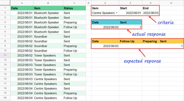
See the ‘actual response’ on the image. You can see two blank columns, i.e., “Follow Up” and “Preparing,” are missing.
How to get the ‘expected response’, i.e., to retain all column labels in Query Pivot?
Helper Range to Add to Query Data
Of course, we will move the date criteria to the outer Query as it applies to the column in the Select clause, i.e., A1:A.
Regarding the condition to apply in column range B1:B, we should follow a workaround. Here it is.
First of all, get the UNIQUE values in the Pivot column C. For that, key in the below formula in K1.
=unique(C2:C)It will return three unique values and that is “Sent,” “Preparing,” and “Follow up.” Please refer to the below image.
Use the below SUBSTITUTE formula in J1 to repeat the E2 criterion thrice.
=ArrayFormula(SUBSTITUTE(E2,"",sequence(counta(K1:K))))Then the below SUBSTITUTE formula in I1 will repeat the G2 (end-date) criterion +1 thrice.
=ArrayFormula(SUBSTITUTE(G2+1,"",sequence(counta(K1:K))))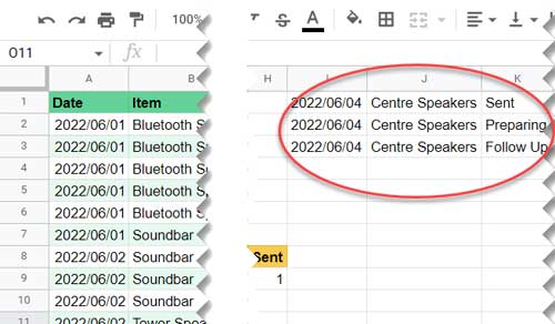
Why should we add +1 to the end date?
The source data is in A1:C. Instead, we will use {A2:C;I1:K} as the source data.
The +1 to the end date will later help us exclude the helper range from the Query response.
Actually, the above helper formulas will help us retain all column labels in the Pivot table in Query.
We can use the below formula (E8), which will retain the missing column labels in Query Pivot.
=query(Query({A2:C;I1:K},"Select Col1,Count(Col2) where Col2='"&E2&"' group by Col1 pivot Col3 label Col1 'Date'",0),"Select * where Col1 >= date '"&text(F2,"yyyy-mm-dd")&"' and Col1 <= date '"&text(G2,"yyyy-mm-dd")&"'")The column 2 condition is within the first query.
Regarding the column 1 conditions, you can find them within the outer Query.
That’s all. Thanks for the stay. Enjoy!