


")


")

")
")
 in Excel & Google Sheets")


In this tutorial, you’ll learn how to easily retain all column labels in a Query Pivot in Google Sheets, ensuring your data stays organized and easy to understand, no matter how complex your dataset is.
When working with Google Sheets, the QUERY function with the PIVOT clause allows you to create flexible pivot tables without relying solely on the built-in Pivot Table tool (Insert > Pivot Table). It’s a powerful way to summarize and analyze data.
However, a common issue users face is losing column labels when pivoting data, which can lead to unpredictable columns and misinterpretation of results.
The easiest way to solve this problem is to understand why column labels go missing. Let’s dive in.
This guide is part of the QUERY Pivot & Reporting in Google Sheets hub and explains how to retain all pivot column labels, even when no matching data exists.
Reason for Missing Column Labels in Query Pivot
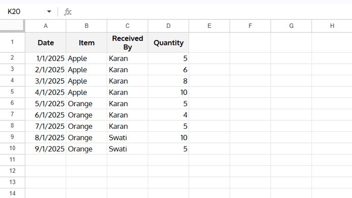
Assume both Karan and Swati have received items from vendors, and the source data is structured as follows:
| Date | Item | Received By | Quantity |
|---|---|---|---|
| 1/1/2025 | Apple | Karan | 5 |
| … | … | … | … |
| … | … | … | … |
When you group the data by Item and pivot by Received By, the items appear as row labels and the recipients (Karan, Swati) appear as column labels:
| Item | Karan | Swati |
|---|---|---|
| Apple | … | … |
| Orange | … | … |
If you then filter the items—for example, by using a WHERE clause to select only Apple—any recipient who has not received that item will no longer appear as a column label. This happens because the WHERE clause filters out their rows before the PIVOT operation is applied.
Note: This behavior is not specific to QUERY pivots; it also applies to standard Pivot Tables in Google Sheets.
Examples of Retaining All Column Labels in Query Pivot
We’ll explore two examples to help you retain all column labels in a QUERY pivot. The technique varies depending on whether your filter applies to a column in the SELECT clause or additional columns.
Sample Data for QUERY Pivot Examples
Example 1: Filtering Applied to SELECT Clause Column
Scenario: You want to filter Apple while summing ‘Quantity’ and pivoting ‘Received By.’
Regular query formula:
=QUERY(A1:D,"SELECT Col2, sum(Col4) WHERE Col2 ='Apple' GROUP BY Col2 PIVOT Col3")Result:
| Item | Karan |
| Apple | 29 |
Problem: Swati is missing because she hasn’t received Apple.
Solution: Move the filter outside with a nested query:
=QUERY(
   QUERY(A1:D, "SELECT Col2, sum(Col4) WHERE Col2 IS NOT NULL GROUP BY Col2 PIVOT Col3"),
   "SELECT * WHERE Col1='Apple'"
)
Result:
| Item | Karan | Swati |
| Apple | 29 |
How it works:
- Inner query generates the pivot table for all items.
- Outer query filters only the desired item (
Apple). - This ensures all recipients remain as column labels.
Example 2: Filtering SELECT Clause Column + Additional Column
Scenario: You want to filter Apple and a date range (not in SELECT clause).
Steps:
- Enter
Applein F1, start date in G1, end date in H1. - Regular query formula:
=QUERY(A1:D, "SELECT Col2, sum(Col4) WHERE Col2='Apple' AND Col1>= date '"&TEXT(G1,"YYYY-MM-DD")&"' AND Col1<= date '"&TEXT(H1,"YYYY-MM-DD")&"' GROUP BY Col2 PIVOT Col3")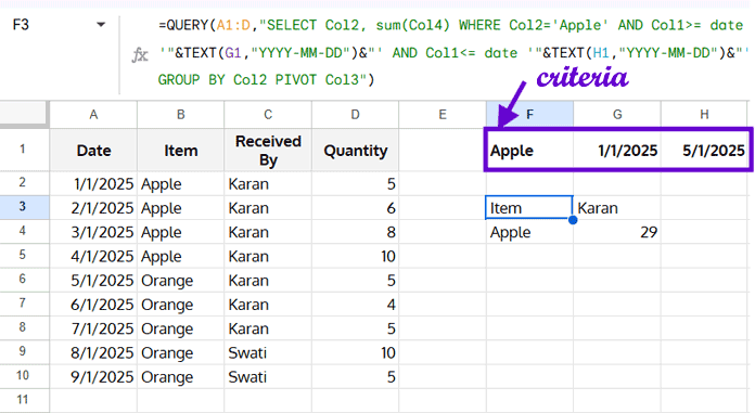
Problem: Swati is missing if she didn’t receive Apple during the selected date range.
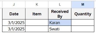
Solution: Use a helper table stacked with the original data:
- Prepare a helper range (
J1:M) matching the size ofA1:D. - In the pivot column (third column), enter all unique recipient names using the following formula in L2:
=UNIQUE(C2:C)- In the date column (first column of helper), enter a date within the start-end range.
- Stack with
VSTACK:
=QUERY(
   QUERY(VSTACK(A1:D, J2:M),
      "SELECT Col2, sum(Col4) WHERE Col1>= date '"&TEXT(G1,"YYYY-MM-DD")&"' AND Col1<= date '"&TEXT(H1,"YYYY-MM-DD")&"' GROUP BY Col2 PIVOT Col3"
   ),
   "SELECT * WHERE Col1='Apple'"
)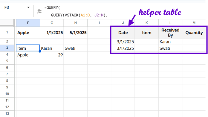
Result: Both Karan and Swati appear as column labels, even if Swati has no transactions in the filtered date range.
Conclusion: Retaining All Column Labels Made Easy
By following these two examples, you can retain all pivot column labels in QUERY.
The key is:
- Filter columns in the SELECT clause are applied outside the inner query.
- Filters on other columns require a helper range stacked with the data to preserve all labels.
Key Takeaways
- QUERY pivot tables may lose column labels if filtered.
- Use nested queries to apply filters after pivoting.
- Helper tables ensure additional filters do not remove column labels.
- This method keeps your pivot tables accurate and readable.