My project duration is from 01/04/2019 to 31/12/2019. How to start counting week number from 01/04/2019 instead of 01/01/2019? I want to reset week number in Google Sheets for April first week to 1 and continue the counting till the end of the year.

In the above example, the month, which I have specified, may not necessarily be April. It can be a different month.

In a different scenario, I want to reset the week number for every month. Is there an efficient solution to these problems without using a script?

Yes! We can start counting week number 1 from any month and date in Google Sheets using the WEEKNUM function.

Let us begin with a basic example to reset week number in Google Sheets. After that, I can provide you an array formula to reset week number of a range.

Of course, the formula will be different for resetting week count for every month and resetting week count for a specific month.

The function WEEKNUM is the key in my formulas. See the syntax first.

WEEKNUM(date, [type])

You can refer to my How to Utilise Google Sheets Date Functions to learn more about the WEEKNUM function.

How to Reset Week Number for a Specific Month

In cell D3 I have keyed in the date 01/04/2019. It’s in dd/mm/yyyy format as per my Sheets’ locale settings. You may enter the date as per your Google Sheets’ locale settings (File > Spreadsheet settings > General > Locale).

If you use the below WEEKNUM formula, you will get the week count as 14. Because the date 01/04/2019 falls in 14th weeks of the year.

=weeknum(D3)

I want to reset this week number 14 to 1. I will explain to you how to properly reset the week number in any specific month or date in Google Sheets.

You can normally use this non-array formula to reset the week number of a specific month.

Non-Array Formula # 1:

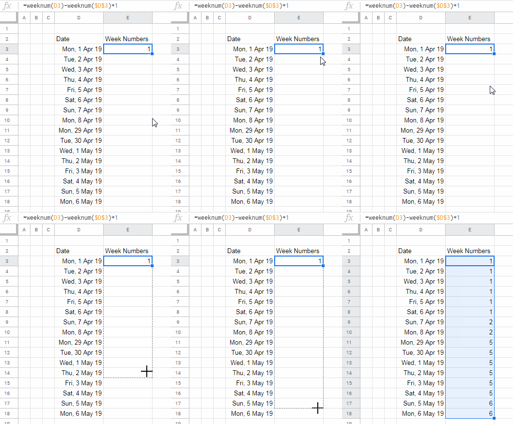
=weeknum(D3)-weeknum($D$3)+1

You can convert the above custom week count formula in cell E3 to an auto-expanding array formula. Why it is necessary?

I have my project start date in cell D3 as 01/04/2019. The project ends on 31/12/2019. So I have a long list of dates in D3:D. In that case, you can convert the above formula to an array formula.

Array Formula # 1:

=ArrayFormula(if(len(D3:D),weeknum(D3:D)-weeknum($D$3)+1,))

Explanation:

• ArrayFormula – To expand the result (make non-array to an array).
• LEN – Return output only if D3:D contains values.

Additional Tips – ‘Types’ in Weeknum Count

In the above example, I have considered day week begins on Sunday and ends on Saturday. I have achieved this by omitting the ‘type’ argument in the WEEKNUM function (please refer the syntax).

By default, the ‘type’ is 1 and that means “Sunday – Saturday”. You can use different defined numbers to use different week start and end days.

If you consider your day week beings on Monday and ends on Sunday, then modify the above week number resetting formula as below.

Non-Array Formula # 2:

=weeknum(D3,2)-weeknum($D$3,2)+1

Array Formula # 2:

=ArrayFormula(if(len(D3:D),weeknum(D3:D,2)-weeknum($D$3,2)+1,))

I have included the ‘type’ as 2 in the formula. You can refer to this Docs Editors Help to know more about the ‘Type’ available to control the week start and end days.

Reset Week Number for Every Month in Google Sheets

How to reset the week number count to 1 for the beginning of every month?

Non-Array Formula # 3:

=weeknum(D3)-weeknum(date(year(D3),month(D3),1))+1

Compared to the Non-Array Formula # 1, here I have changed cell $D$3 inside the WEEKNUM to date(year(D3),month(D3),1) which would dynamically return the month start date in each row.

Array Formula # 3:

This array formula follows the same logic above.

=ArrayFormula(if(len(D3:D),weeknum(D3:D)-weeknum(date(year(D3:D),month(D3:D),1))+1,))

You can follow this method to reset week number count for every month in Google Sheets. Here also you can use the ‘type’ argument as per Non-Array Formula # 2 and Array Formula # 2.

Starting Week Number Count from a User-Specified Date

Assume your project or any activity start date is 18/07/2019. You want to count the week number from this date and the count should start from 1.

Here are the steps to reset week number based on a user-specified date.

Step 1:

Find the day of the week of the date 18/07/2019 which is in cell D2. We can use the TEXT function for this.

=text(D3,"dddd")

Result: Thursday

Step 2:

Find the ‘Type’ (defined number) of the week starting with Thursday as week start day (Thursday – Wednesday). You can see that it’s 14.

Note: To find this number you can check WEEKNUM function in my Google Sheets Functions Guide.

Step 3:

At this point, we can copy the Non-Array Formula # 1 above and modify it as below.

Non-Array Formula # 4:

=weeknum(D3,14)-weeknum($D$3,14)+1

I have used the ‘type’ 14 in the WEEKNUM function here.

Can I convert this formula to an array?

No doubt, you can follow the earlier array formulas especially the Array Formula # 1 here.

Array Formula # 4:

=ArrayFormula(if(len(D3:D),weeknum(D3:D,14)-weeknum($D$3,14)+1,))

Time to conclude this topic of how to reset the week number in Google Sheets. Please let me know if you have any questions/comments. Enjoy!