In this tutorial, I’ll share one unique and dynamic way to repeat a single column or multiple columns (table) n times in Google Sheets using VLOOKUP as the key function.
My approach involves leveraging SEQUENCE within the is_sorted argument of VLOOKUP for horizontally repeating columns in Sheets.
VLOOKUP is typically used to search for a key in the first column of a range. However, there is a clever way to duplicate a column n times. For multiple columns, we will also utilize the REDUCE lambda function.
These are novel ideas with two benefits:
- The formulas never use the SPLIT function, so no concatenating takes place in repeating columns.
- The formulas are dynamic, allowing you to increase or decrease the repetition simply by specifying ‘n’.
Let’s explore this innovative approach to repeating columns horizontally in Google Sheets.
Purpose of Repeating Data Horizontally
When you want to print labels, you might find repeating a single column ‘n’ times useful. This allows you to utilize the maximum paper area when printing.
Imagine you manage a sales team and need to prepare monthly sales reports. Each month’s report has the same structure. By repeating multiple columns, such as a table, you can prepare a comprehensive annual report that shows each month’s data side by side.
How to Repeat a Column N Times Horizontally in Google Sheets
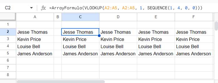
In the following example, I want to repeat the names in the range A2:A5 horizontally four times. Here is the formula to do that:
=ArrayFormula(VLOOKUP(A2:A5, A2:A5, 1, SEQUENCE(1, 4, 0, 0)))In this formula, 4 represents the number of repetitions (n), and A2:A5 represents the column range to repeat.

How does this formula work?
Syntax:
VLOOKUP(search_key, range, index, [is_sorted])The VLOOKUP function is commonly used for vertical lookup. It searches for a key in the first column of a range and returns a value from a specified column (by index) in the range.
When you specify multiple search keys and use ARRAYFORMULA, VLOOKUP searches for all these values and returns corresponding values from the same or another column in the range.
Explanation:
In our example, by specifying A2:A5 as both the search_key and range, and 1 as the index number, the formula returns the same column values.
How do we repeat it?
We use the is_sorted argument for that purpose. It uses 0 (exact match) or 1 (approximate match, but only with a sorted range).
Here’s the key point: you specify is_sorted as many times as you want to repeat the column. For instance, if you want to repeat the column 4 times horizontally, you should specify four 0s.
In our formula, the SEQUENCE function generates four 0s.
How to Repeat Multiple Columns (a Table) N Times Horizontally in Google Sheets
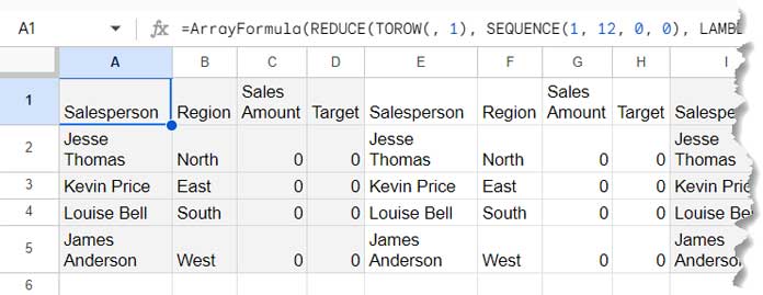
I have the following data structure for monthly sales reports in cell range A1:D5 in “Sheet1”. In “Sheet2”, I want a formula in cell A1 that will repeat this table 12 times:
| Salesperson | Region | Sales Amount | Target |
| Jesse Thomas | North | 0 | 0 |
| Kevin Price | East | 0 | 0 |
| Louise Bell | South | 0 | 0 |
| James Anderson | West | 0 | 0 |
Once repeated, I’ll copy the result and paste it as values, then fill in the “Sales Amount” and “Target” columns.
This approach allows me to track each month’s performance while keeping the data organized and easily comparable across the year.
To repeat multiple columns horizontally, we will use an extended version of VLOOKUP.

Formula:
=ArrayFormula(REDUCE(TOROW(, 1), SEQUENCE(1, 12, 0, 0), LAMBDA(a, v, HSTACK(a, VLOOKUP(Sheet1!A1:A5, Sheet1!A1:D5, SEQUENCE(1, 4), v)))))When using this formula, make the following changes:
Replace:
Sheet1!A1:A5with the first column reference in the range,Sheet1!A1:D5with the range to repeat,12in the first SEQUENCE with the number of times to repeat the range,4in the second SEQUENCE with the number of columns in your range.
Formula Breakdown
The following VLOOKUP formula returns the specified range:
=ArrayFormula(VLOOKUP(Sheet1!A1:A5, Sheet1!A1:D5, SEQUENCE(1, 4), 0))It searches for keys in Sheet1!A1:A5 within the first column of Sheet1!A1:D5 and returns values from columns 1 to 4, defined by SEQUENCE(1, 4).
In the previous formula, we specified is_sorted as 0 to repeat a single column that many times.
Following the same logic, if you specify it as:
=ArrayFormula(VLOOKUP(Sheet1!A1:A5, Sheet1!A1:D5, SEQUENCE(1, 4), SEQUENCE(1, 12, 0, 0)))The formula will return values for the specified 4 columns, while the remaining 8 columns will contain #N/A errors.
To address this, we utilize the REDUCE function, which reduces an array to an accumulated result by applying a LAMBDA function to each value.
The approach involves feeding is_sorted with 0 one at a time.
The VLOOKUP result is stored in an accumulator, which initially holds a null value. We use HSTACK to horizontally stack the accumulator value with the VLOOKUP result in each iteration.
Syntax:
REDUCE(initial_value, array_or_range, LAMBDA)initial_value:TO_ROW(, 1)represents null.array_or_range:SEQUENCE(1, 12, 0, 0)is used in theis_sortedargument.lambda:LAMBDA(a, v, HSTACK(a, VLOOKUP(Sheet1!A1:A5, Sheet1!A1:D5, SEQUENCE(1, 4), v)))is the lambda function.
The REDUCE function iterates 12 times (array_or_range) with a lambda function.
In this lambda function, a represents the accumulator (initially null), and v represents the current iteration number (1 to 12).
HSTACK stacks the accumulator value with the VLOOKUP result in each iteration. The final output will repeat multiple columns, specifically Sheet1!A1:D5, 12 times.


Great article – thanks for the context. Can you use it within a more complicated formula? I’m trying to use a sequence to return doubles of the same date. Can’t seem to get this to work…
Hi, Julian,
I think I can do that. If possible, make an example Sheet. Let me ‘VIEW’ your sample data and the result.
Best,
I am glad that you liked it.
Regarding your question you may please consider sharing a sample sheet and also on that sheet please manually enter the output you expect.
Thanks.
Hi Prashanth! Great Article, explained in a simple and clear manner! Quick question, how can I multiply using an array. Example: I have two columns.. in the Twitter, Wikipedia example of yours, next to it I have the number of times I want to multiply each twitter, wikipedia, etc… correspondingly… the result should be in one column only… how can I use one formula for this?