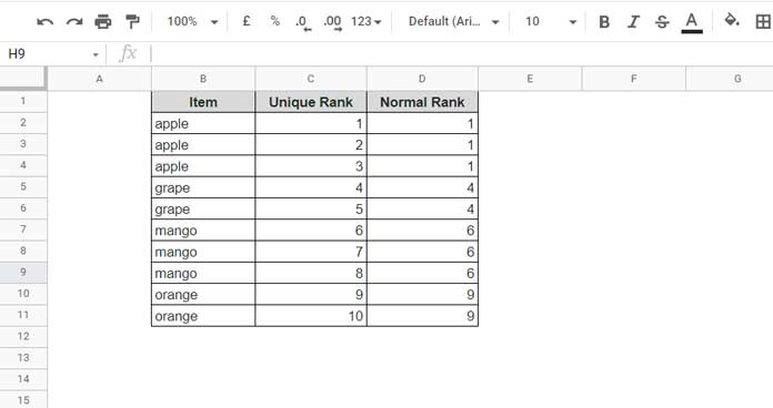
When you rank text values in Google Sheets, duplicates normally receive the same rank. For example, in the table below, every “apple” is ranked 1, which can be fine in some cases — but not when you need unique ranks for each entry.
Sorted list example:

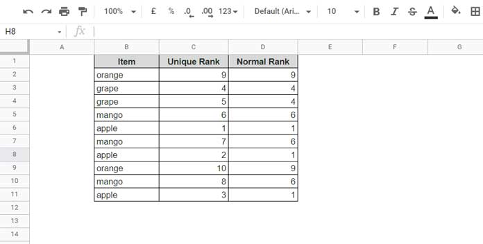
Even in an unsorted list, the issue remains — ties get the same number, leaving gaps in the ranking sequence.
Unsorted list example:

In this tutorial, you’ll learn how to rank text uniquely in Google Sheets, so each item gets its own rank number, even if there are duplicates.
Why the Regular Alphabetical Ranking Formula Doesn’t Work
A normal alphabetical ranking formula gives the same rank to duplicates — “apple” at #1 for every occurrence. For unique ranks, each duplicate needs its own number: first “apple” gets #1, second gets #2, and so on.
How This Works (Concept Overview)
Whether your list is sorted or unsorted, the idea is the same.
We combine two counts:
- Count of Text Below – How many items are alphabetically less than the current item.
- Running Count of Text – The position of the current item among duplicates.
Generic Formula:
Unique Rank of Text = Count_of_Text_Below + Running_Count_of_Text
Example with a Sorted List
Sample Data
| Item | Count_of_Text_Below | Running_Count_of_Text | Unique Rank of Text |
|---|---|---|---|
| apple | 0 | 1 | 1 |
| apple | 0 | 2 | 2 |
| apple | 0 | 3 | 3 |
| grape | 3 | 1 | 4 |
| grape | 3 | 2 | 5 |
Explanation:
- For
"apple", there are no items less than it, soCount_of_Text_Below = 0. - For
"grape", there are 3 apples less than it, soCount_of_Text_Below = 3.
The Running Count just counts each duplicate’s position in sequence.
Formula to Rank Text Uniquely in Google Sheets (Non-Array Version)
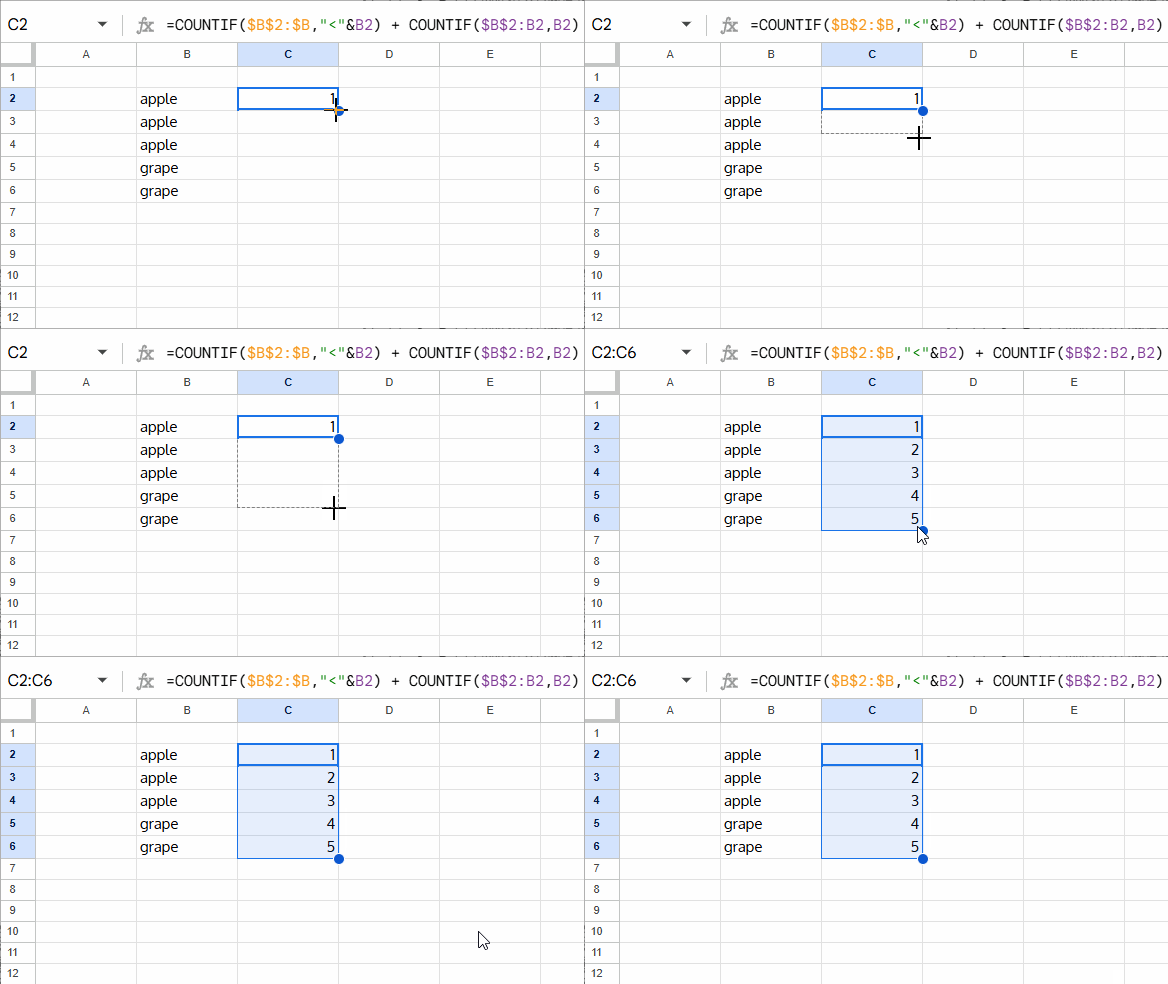
If you want to use a standard drag-down formula:
=COUNTIF($B$2:$B,"<"&B2) + COUNTIF($B$2:B2,B2)
Parts of the formula:
COUNTIF($B$2:$B,"<"&B2)→ Count of text belowCOUNTIF($B$2:B2,B2)→ Running count of the text
Works on both sorted and unsorted lists.
Formula to Rank Text Uniquely in Google Sheets (ArrayFormula Version)
If you prefer a single ArrayFormula that auto-fills down:
=ArrayFormula(
  IF(B2:B="",,
    COUNTIF(B2:B,"<"&B2:B) +
    COUNTIFS(B2:B,B2:B,ROW(B2:B),"<="&ROW(B2:B))
  )
)
Breakdown:
COUNTIF(B2:B,"<"&B2:B)→ Count of text belowCOUNTIFS(B2:B,B2:B,ROW(B2:B),"<="&ROW(B2:B))→ Running count of textIF(B2:B="",,)→ Prevents output in blank rows
Why This Method is Reliable
- Works on sorted or unsorted lists
- Handles any number of duplicates correctly
- Fully compatible with Google Sheets’ dynamic array behavior


