


At present, to calculate the percentile for each group, there is no dedicated function in Google Sheets.
We can use a combination of either of the FILTER or IF with PERCENTILE for the same.
Why should one want to calculate group-wise percentile (group-wise centile) in Google Sheets?
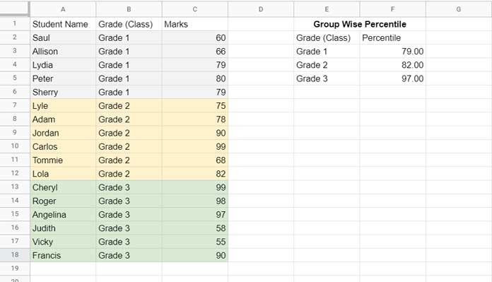
Assume you have a table that contains marks of students in two different grades (classes).
To get the 75% centile of all the marks, you can straightaway use the PERCENTILE function.
Syntax: =percentile(all_marks,0.75)
But when you want to calculate the centile for each grade (class), then the function alone won’t work. Here we can use the said combination.
I hope, you could understand the term group-wise percentile in Google Sheets.
Before going to an example that contains marks and grades, here are a few more details.
You may be familiar with the statistical functions AVERAGE, MIN, MAX, MEDIAN, RANK, etc. Unlike these functions, PERCENTILE may not be most common in use.
So, I think it’s wise to give you some idea about this statistical function.
In short, what MEDIAN returns in a numerical dataset will be equal to 50th centile.
For example, the MEDIAN of the numbers 5 and 6 will be 5.5. No doubt, the 50th centile of these numbers will also be the same value.
Also, please note that both the functions interpolate to determine the value at the 50th percentile.
How to Calculate k-th Percentile for Each Group in Google Sheets
k-th: The percentile value in the range 0 to 1 (0% to 100%), inclusive (for example, you can specify 0.6 or 60% as the k-th percentile).
Sample Data: A1:C
To get the 60th centile of all the marks, we can use the below formula.
=percentile(C2:C18,0.6)Result: 81.20
It means, 81.20 is the 60th percentile mark in this set. We can say 60 percent of students scored below 81 marks.
Group Wise Percentile in Google Sheets
Please refer to the image above for the result in the cell range F3:F5. Here are the steps to follow.
Steps:-
1. The first step here is to get the group (here grades in column B) without duplicates. For that, insert the below UNIQUE formula in cell E3.
=sort(unique(B2:B))It will return the grades;
Grade 1, Grade 2, and Grade 3.
2. Now we can start calculating the percentile for each of these Groups in Google Sheets. For that, as I have mentioned, we can use a combination of FILTER and PERCENTILE functions.
Key the below formula in cell F3 and drag-down to F4 and F5.
=percentile(filter($C$2:$C,$B$2:$B=E3),0.6)The FILTER formula filters the marks in C2:C based on the Grade in E3, i.e., $B$2:$B=E3. The PERCENTILE then returns the 60th centile of this filtered group.
This PERCENTILE and IF combination will also serve the purpose.
=ArrayFormula(percentile(if($B$2:$B=E3,$C$2:$C),0.6))Here the IF formula returns the marks if the Grade matches, else FALSE.
Creating a Percentile Column
Here is one more example. Here we are calculating the percentile for each group in a new column for all the rows.
Didn’t get it?
Please see column D in the below example.
The change is in the FILTER formula criterion part.
In the above example, the FILTER uses the UNIQUE output as the criterion to filter the marks. Here instead, it uses the condition from the table (column B) itself.
=percentile(filter($C$2:$C,$B$2:$B=B2),0.6)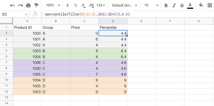
Note:– For the calculation, the data doesn’t need to sort.
That’s all.
Thanks for the stay. Enjoy!
Resources: