")


")


")

")
")
 in Excel & Google Sheets")


We can take the help of the LET function to simplify the formula that calculates the percentage of grand total in the Google Sheets QUERY function. But before jumping into that, let me show you how to do the same using a Pivot Table. Because, honestly, Pivot Table is the easiest method.
Then, you might ask—why use QUERY? The reason is simple: when you want more flexibility and the ability to create pivot charts, the better option is the QUERY function.
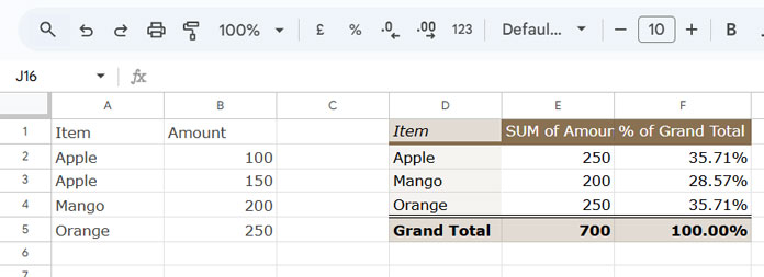
How to Properly Display the Percentage of Grand Total in a Pivot Table
For this example, I’m using a small dataset with five rows (including the header row), like this:
Follow these five steps to group the data and display the percent of grand total using a Pivot Table:
Steps
- Select the range
A1:B5. (If your range is different, select accordingly.) - Click Insert > Pivot table.
- Check Existing Sheet and enter a cell address, for example,
D1. - Click Create.
- In the Pivot Table Editor:
- Add
Itemunder Rows. - Add
Amountunder Values. - Ensure Summarise by is set to SUM (this is usually the default).
- Add
Amountagain under Values. - For the second
Amount, under Show as, select % of grand total.
- Add
That’s all.
Tip: You can click on cells E1 and F1 in the Pivot Table to modify the field labels.
That’s how we display the percentage of grand total in a Pivot Table.
How to Calculate the Percentage of Grand Total Using the QUERY Function
Let’s now go step-by-step using the QUERY function. To summarize the data by item, like in the Pivot Table above, use this formula:
=QUERY(A1:B, "SELECT Col1, SUM(Col2) WHERE Col1 IS NOT NULL GROUP BY Col1", 1)This formula returns:
| Item | sum Amount |
| Apple | 250 |
| Mango | 200 |
| Orange | 250 |
Now, how do we add a percentage of grand total column just like the Pivot Table?
The logic is:
Percent of grand total = Total for each item ÷ Grand total
To achieve this, we’ll use the CHOOSECOLS function to extract columns from the QUERY result, and the LET function to simplify the formula.
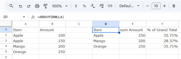
Here’s the formula:
=ARRAYFORMULA(
  LET(
    qry, QUERY(A1:B, "SELECT Col1, SUM(Col2) WHERE Col1 IS NOT NULL GROUP BY Col1", 1),
    col_1, CHOOSECOLS(qry, 1),
    col_2, CHOOSECOLS(qry, 2),
    HSTACK(qry, IFERROR(col_2/SUM(col_2), "% of Grand Total"))
  )
)
Formula Breakdown:
QUERY(...): Summarizes the data.col_1andcol_2: Extract individual columns usingCHOOSECOLS.col_2/SUM(col_2): Divides each item’s total by the grand total.IFERROR(..., "% of Grand Total"): Replaces the header row error with a label.HSTACK: Combines the QUERY result with the new percentage column.
Note: You can format the third column by selecting it and choosing Format > Number > Percent.
To rename headers, wrap the formula with another QUERY like this:
=QUERY(
  your_formula,
  "LABEL Col1 'Item', Col2 'Total', Col3 '% of Grand Total'",
  1
)
Add a Grand Total Row to the QUERY Result with Percentage of Grand Total Column
To append a dynamic total row, use this formula. Replace your_formula with the full formula above and set n as the number of text columns (e.g., 1 in this case):
=ArrayFormula(LET(
   ftr, your_formula,
   tc, n,
   VSTACK(ftr, HSTACK("Total", DSUM(ftr, SEQUENCE(1, COLUMNS(ftr)-tc, tc+1), IFNA(VSTACK(CHOOSEROWS(ftr, 1), )))))
))
For a detailed breakdown of this logic, check out my tutorial: Dynamic Total Row for FILTER, QUERY, or ARRAY Results in Sheets
Thank you for this.
Is there a way for this to work with additional where conditions?
For example, if you add
where not(Col1)= 'apple', the orange and mango % will still show the same when they should be 200/(200+250)-mango and 250/(200+250)-orange.Hi, Craig,
You should replace the
sum(C2:C5)withindex(sumif(NE(B2:B5,"apple"),true,C2:C5)).It appears in two places in the formula.
This is great! However, what if I want the total percent by row?
Hi, Philip Rinehart,
An example sheet, please.