Flattening in Google Sheets helps you arrange multiple columns into a single column. Sometimes, however, you don’t want to flatten the entire dataset—only specific columns. Partially flattening a multi-column array in Google Sheets lets you transform your data into a more manageable, vertical layout while keeping key information intact. In this tutorial, you’ll learn how to flatten only the columns you need, making it easier to analyze, summarize, or use in formulas.

Introduction: Why Partially Flatten a Multi-Column Array?

Imagine you have data in four columns:

• Column A contains descriptions of construction activities (tasks).
• Columns B, C, and D hold week-wise completion weightage.

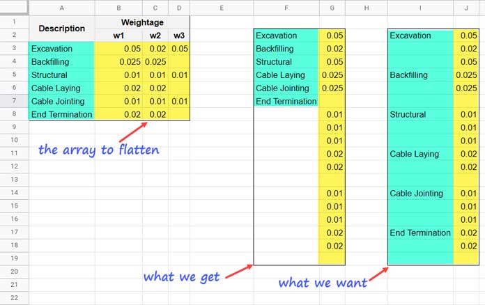
You might want to partially flatten a multi-column array in Google Sheets so that only the weightage columns are stacked vertically, while the task names remain properly aligned.

The final output will have just two columns: Activities and Weightage.

A typical but unsuccessful attempt looks like this:

F2: ={A3:A8}
G2: =FLATTEN(B3:D8)

As you’ll see, the flattened weightage won’t align with the tasks.

Example 1: Partially Flatten Two Columns

To align tasks with their weightage, use these formulas:

I2: =ArrayFormula(FLATTEN({A3:A8, IFERROR(A3:B8/0)}))
J2: =FLATTEN(B3:D8)

Pro Tip: You can combine them into one formula:

=ArrayFormula({FLATTEN({A3:A8, IFERROR(A3:B8/0)}), FLATTEN(B3:D8)})

However, using two steps is more flexible if you want to leave multiple columns untouched.

How the Formula Works

• FLATTEN({A3:A8, IFERROR(A3:B8/0)}) creates virtual blank cells below each task.
• IFERROR(A3:B8/0) generates blank columns without causing errors.
  Note: If you want to partially flatten three columns, the IFERROR(.../0) part should include two columns of the same size as the column you want to keep intact. In general, the number of “virtual blank” columns should be one less than the total number of columns being flattened to maintain proper alignment.
• ArrayFormula ensures the operation applies to the entire range.

This is the key to partially flatten a multi-column array in Google Sheets while keeping your tasks aligned with their corresponding data.

Handling Dynamic Ranges

If your data grows over time (like A3:A or B3:D), wrap the ranges in FILTER to ignore empty rows:

I2: =FLATTEN({FILTER(A3:A, A3:A<>""), FILTER(IFERROR(A3:B/0), A3:A<>"")})
J2: =FLATTEN(FILTER(B3:D, A3:A<>""))

Example 2: Partially Flatten Three Columns

Sometimes, you might want to insert an additional column for total weightage. In that case:

• Flatten the last three columns (C3:E8) in I3.
• Insert blank cells for task names in G3:

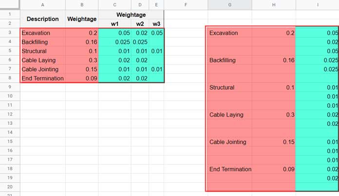
G3: =ArrayFormula(FLATTEN({A3:A8, IFERROR(A3:B8/0)}))
I3: =FLATTEN(C3:E8)

To align the second column (B3:B8), insert blank cells like this:

H3: =ArrayFormula(FLATTEN({B3:B8, IFERROR(A3:B8/0)}))

Flattening More Columns with VLOOKUP

If you need to keep several columns intact on the left, a VLOOKUP array formula works well. In the example above, you can replace the H3 formula with this:

=ArrayFormula(IFNA(VLOOKUP(G3:G18, A3:B8, {2}, 0)))

• This searches tasks in G3:G18 and returns values from B3:B8.
• Change {2} to {2,3} to return multiple columns at once.

This approach makes it easier to partially flatten a multi-column array in Google Sheets without losing alignment.

Wrapping Up

That’s it! Now you know how to partially flatten a multi-column array in Google Sheets, whether you’re flattening two, three, or more columns. These techniques help you maintain proper alignment, create flexible layouts, and make your data ready for analysis or reporting.

Enjoy experimenting with your sheets, and happy flattening!

Resources

• How to Flatten Every Other Column in Google Sheets
• Unpivot Data in Google Sheets (Reverse Pivot Formula Explained)
• How to Unstack Data into Groups in Google Sheets
• How to Stack Data in Google Sheets: Tips and Tricks
• Unstack Multiple Form Responses in Google Sheets
• 3-Column Hierarchical Table in Google Sheets (No Scripts!)
• EXPAND + Stacking: Expand an Array in Excel