There isn’t a single universal formula for performing a partial match between two columns in Google Sheets. The approach depends on the specific requirements. Let’s explore this with the following example data in columns A and B:
| Description (Column A) | Item (Column B) |
| Adjustable Standing Desk | Steel |
| Stainless Steel Water Bottle | Stainless Steel |
| Ortho Chair | Chair |
| Recliner Sofa | Sofa |
| Wireless Bluetooth Headphones | Bluetooth |
| 4K Ultra HD Smart TV | Ultra |
| Ergonomic Office Chair |
Problem Scenarios
- Match the word “Steel” (the first item in column B) in column A and return the partially matching description.
- Match the phrase “Adjustable Standing Desk” (the first item in column A) with values in column B by identifying any word from the phrase and returning the corresponding values.
These scenarios require different formulas. Let’s go through the solutions step by step.
Find Partial Matches in Two Columns and Return Matching Items
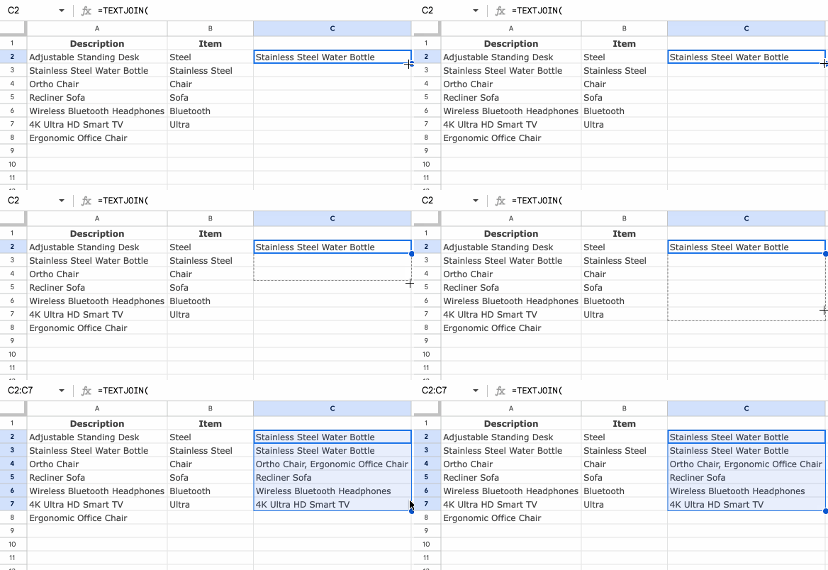
To solve the first scenario, where you want to match the keyword in column B with descriptions in column A, use the following formula:
=TEXTJOIN(
   ", ",
   TRUE,
   IFNA(
      FILTER($A$2:$A, ISNUMBER(SEARCH(B2, $A$2:$A)))
   )
)
Enter this formula in cell C2 and drag it down to match all values in column B with the corresponding values in column A.

Formula Breakdown:
SEARCH(B2, $A$2:$A): Finds the keyword inB2within columnAand returns a number (if found) or an error (if not found).ISNUMBER(...): Converts results toTRUEfor matches (numbers) andFALSEfor mismatches (errors).FILTER($A$2:$A, ISNUMBER(...)): Filters columnAto include only the matching rows.IFNA(...): Removes errors if no match is found.TEXTJOIN(", ", TRUE, ...): Combines results into a single string, separated by commas.
Issue: This formula may return undesired matches for substrings (e.g., “and” matching “brand” or “ampersand”). For exact word matches, use the next formula.
Exact Word Matches in Google Sheets
Use this formula to ensure only exact word matches are returned:
=TEXTJOIN(
   ", ",
   TRUE,
   IFNA(
      FILTER($A$2:$A, REGEXMATCH($A$2:$A, "(?i)\b(" & B2 & ")\b"))
   )
)Explanation:
REGEXMATCH($A$2:$A, "(?i)\b(" & B2 & ")\b"): Matches the exact word inB2within columnA(case-insensitive).- The rest of the formula components function similarly to the previous example.
Match Any Word from a Phrase in One Column with Another Column
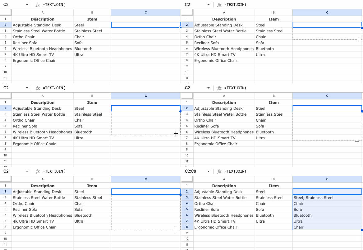
To solve the second scenario, where you match any word from a phrase in column A with values in column B, use this formula:
=TEXTJOIN(
   ", ",
   TRUE,
   IFNA(
      FILTER($B$2:$B, REGEXMATCH($B$2:$B, "(?i)" & TEXTJOIN("|", TRUE, "\b(" & SPLIT(A2, " ") & ")\b")))
   )
)
Drag this formula down as needed to process multiple rows.
Explanation:
SPLIT(A2, " "): Splits the value inA2into individual words."(?i)" & TEXTJOIN("|", TRUE, "\b(" & SPLIT(A2, " ") & ")\b"): Joins the words into a regular expression pattern for word matching.REGEXMATCH($B$2:$B, ...): Matches any word fromA2in columnB.- The rest of the formula works as described in previous examples.
Conclusion
We explored three formulas to handle different types of partial matches between two columns in Google Sheets:
- Basic partial match using SEARCH
- Exact word match using REGEXMATCH
- Matching any word from a phrase using SPLIT and REGEXMATCH
Choose the formula based on your specific requirements.


Thank you.
This solution works like a charm.
Much obliged.
Hi,
I want to have in C or any other column, a clean list of Column A filtered out with the text in B column.
Thanks (my current method is making helper columns, copy, and paste, etc.)
Hi, SPH,
This may help – Filter Out Matching Keywords in Google Sheets – Partial or Full Match.
Hello. This formula seems to be exactly what I need. However, it is not capturing partial matches. So, if column A includes “orange” and B contains “orange juice” the response is “No”. My understanding is that it would be “Yes” because it does contain “orange”.
=ArrayFormula(if(len(B2:B),if(COUNTIF(A2:A,"*"&B2:B&"*")>=1,"Yes","No"),))Also, would it match “oranges” which include “orange” within the larger plural word?
Thank you!
Hi, Jason,
Maybe this.
=ArrayFormula(if(len(A2:A),if(COUNTIF(B2:B,"*"&A2:A&"*")>=1,"Yes","No"),))Best,
Hello. Thank you for the quick response. Unfortunately, this does not work at all. Yours is the only website I’ve found that comes close to answering my question. I appreciate your help!
HI again. A friend came up with this. Works like a charm:
=filter(Example!B2:B,regexmatch(Example!B2:B,textjoin("|",1,Example!A2:A))=FALSE)Hi, Jason,
Sorry! My answer was without seeing your data.
Please do a search for the key “regexmatch” on this site. You can use the search icon on the top (navigation/menu bar).
Cheers!
Search for a Google Sheet add-on called Flookup. It’s patterned after VLOOKUP with a specific focus on fuzzy or approximate matching… and it’s free
Hello.
I sincerely appreciate your lectures. However, I am having a challenge with your formula in (A) above. I keep getting the error:#NAME?.
The figures is more or less the same as in column D in the 2nd excel example above. Please, how do I fix this?
Thanks
Hi Hakeem,
Please leave a demo sheet.