 in Google Sheets")

")

")


")


")


Google Sheets introduced multiple-selection drop-down chips that allow you to select multiple values from a drop-down list. This feature presents some challenges. The selected items appear as chips within a cell. How do you separate them, aggregate them, and more? I’ll address those issues in this tutorial.
Creating a Multiple-Selection Drop-Down List in Google Sheets
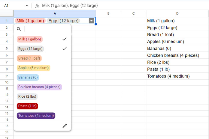
In this example, I will create a multiple-selection drop-down list in cell A1 using the values in column D.
The goal is to make all the values in column D available for selection in cell A1.
Steps:
- Prepare your sample data by entering the values in column D that you want to include in the multiple-selection drop-down list. For this example, assume the data is in the range D1:D9.
- Navigate to cell A1.
- Click on Insert > Drop-down.
- Under “Criteria,” select Drop-down (from a range).
- Enter the range that contains your list in column D, such as
D1:D9. If you want the drop-down list in A1 to include any future values added to column D, enterD:Dinstead. - Select Allow Multiple Selections.
- Click Done.
You have now created a multiple-selection drop-down list in cell A1. You can copy and paste this cell to any other cell as needed. For example, you can copy A1 and paste it into A2:A10 to create the same multiple-selection drop-downs in those cells.
Note: If you prefer not to use the list in column D, you can enter the values manually when creating the drop-down. In that case, in step 4, select ‘Drop-down’ and enter the values one by one. You can skip step 5.
Selecting and Separating Multiple Values from a Drop-Down List
You can select multiple values from the drop-down list in cell A1. Open the drop-down menu by clicking the down arrow. Then, click on the items you want to select. After making your selections, click outside the drop-down menu to close it.
The selected items will appear as chips in cell A1. You may want to increase the column width or apply text wrapping (Format > Wrapping) to view all the selected items.
Separating Values
Although the selected items appear as chips, they are separated by commas in the underlying data. You can view the actual values by selecting the cell and checking the formula bar. Alternatively, you can use =A1 in any cell to display the values.
To separate the selected values into a column, use the following formula:
=ArrayFormula(TOCOL(SPLIT(A1, ", ", FALSE), 3))If you have multiple drop-downs, for example, in the range A1:A10, replace A1 with A1:A10.
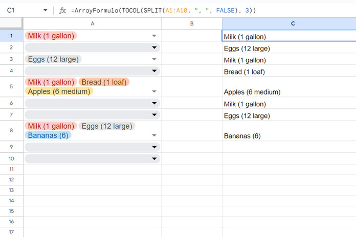
The SPLIT function divides the value in cell A1 using ", " as the delimiter. The TOCOL function then converts the results into a column and removes any empty cells or errors when applied to a range.
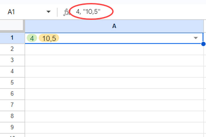
Handling Decimal Separators in Chips
If the decimal separator in your country is a comma and you select the number 10,5 in a drop-down list, the underlying value will be “10,5” (within double quotes).
This won’t cause any issues when separating the multiple-selection drop-down chips into columns. To remove the double quotes, you can use the following formula:
=ArrayFormula(TOCOL(SUBSTITUTE(SPLIT(A1; ", "; FALSE); """"; ""); 3))In this formula, I’ve made two changes compared to the previous one:
- Added the SUBSTITUTE function to replace double quotes with an empty string.
- Changed the argument separators from commas to semicolons. If your decimal separator is a comma, you’ll need to use semicolons as argument separators in the formula.
When using this in a range such as A1:A10 and some cells in this range are blank, the formula will still display blank cells. The TOCOL function won’t remove them because the blank cells contain empty strings returned by the SUBSTITUTE function. If you want to remove them, use the formula as follows:
=LET(flattened; ArrayFormula(TOCOL(SUBSTITUTE(SPLIT(A1:A10; ", "; FALSE); """"; ""); 3)); FILTER(flattened; flattened<>""))The LET function names the formula as flattened and uses that as the range and criteria range in the formula expression part, which is essentially a FILTER formula.
Using COUNTIF with Multiple-Selection Drop-Down Chips
To count a specific item in a multiple-selection drop-down list, you can use the COUNTIF function.
For example, to count occurrences of “Milk (1 gallon)” in the multiple-selection drop-down lists in A1:A, use the following COUNTIF formula:
=COUNTIF(A1:A, "*Milk (1 gallon)*")This COUNTIF formula uses wildcards to match partial text, so any chip containing “Milk (1 gallon)” will be counted.
For an exact match, replace A1:A with the separator formula provided earlier. Here’s an example:
=COUNTIF(ArrayFormula(TOCOL(SPLIT(A1:A, ", ", FALSE), 3)), "Milk (1 gallon)")To get the count of each selected item as a table, use the following QUERY formula:
=QUERY(ArrayFormula(TOCOL(SPLIT(A1:A, ", ", FALSE), 3)), "SELECT Col1, COUNT(Col1) GROUP BY Col1")Any questions about multiple-selection drop-down chips? Feel free to leave them in the comments.
Resources
- Filter Data with Multi-Select Drop-Downs in Google Sheets
- Multiple-Selection Dependent Drop-Downs in Google Sheets
- Multi-Row Dynamic Dependent Drop-Down List in Google Sheets
- Distinct Values in Drop-Down List in Google Sheets
- Create a Drop-Down Menu From Multiple Ranges in Google Sheets
- Relative Reference in Drop-Down Menu in Google Sheets