Multi-condition filtering in the same column refers to applying multiple conditions to one column while filtering rows in a range. This is simple with numeric, time, or date fields using comparison operators, as the FILTER function naturally supports it.
For example, you can filter a range where dates in column A fall between two dates (a date range) or where scores in a column fall between a minimum and maximum score.
But what about filtering a range where the dates in column A fall on more than one specific date or category?
We will discuss this topic in multi-condition filtering in the same column.
Filter Rows Matching Values in a Column Within a Certain Range
We have the following data in A1:C, which represents the delivery dates of a few items:
| Date | Item | Qty |
| 20/07/2024 | Copper Pipes | 5 |
| 20/07/2024 | UPVC Pipes | 4 |
| 23/07/2024 | Brass Fittings | 18 |
| 23/07/2024 | Drain Pipes | 6 |
| 01/08/2024 | Shower Heads | 40 |
| 01/08/2024 | Water Filters | 5 |
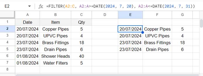
We can use the following FILTER formula to filter the rows in the range where the dates in A2:A fall between 20/07/2024 and 31/07/2024:
=FILTER(A2:C, A2:A>=DATE(2024, 7, 20), A2:A<=DATE(2024, 7, 31))
This follows the syntax FILTER(range, condition1, [condition2, …]).
Where:
range: A2:C – the range to filtercondition1: A2:A>= DATE(2024, 7, 20) – returns TRUE for cells with dates on or after July 20, 2024condition2: A2:A<= DATE(2024, 7, 31) – returns TRUE for cells with dates on or before July 31, 2024
The dates in the conditions are specified as per the DATE function syntax DATE(year, month, day) to avoid issues associated with MM/DD/YYYY or DD/MM/YYYY formats. You can follow the same.
The FILTER function returns rows from the range where the conditions are evaluated to TRUE.
This is how we apply multiple conditions in the same column using the FILTER function in Google Sheets.
Note: You can also use the formula below:
=FILTER(A2:C, ISBETWEEN(A2:A, DATE(2024, 7, 20), DATE(2024, 7, 31)))In this case, the condition is ISBETWEEN(A2:A, DATE(2024, 7, 20), DATE(2024, 7, 31)), which evaluates to TRUE wherever the date falls between the two specified dates, both inclusive. The syntax of ISBETWEEN is:
ISBETWEEN(value_to_compare, lower_value, upper_value, [lower_value_is_inclusive], [upper_value_is_inclusive])The last two optional arguments are TRUE by default.
Filter Rows Matching Specific Values in a Column
In the sample data above, how do we filter the items with delivery dates 20/07/2024 and 01/08/2024?
Please note that the following formula is incorrect:
=FILTER(A2:C, A2:A=DATE(2024, 7, 20), A2:A=DATE(2024, 8, 1))This formula will not work as intended because it cannot simultaneously match both conditions in the same column.
To explain further, condition1, i.e., A2:A = DATE(2024, 7, 20), evaluates to TRUE in certain rows, while condition2, i.e., A2:A = DATE(2024, 8, 1), evaluates to FALSE in those rows, or vice versa.
So, how do we correctly apply multiple conditions in the same column?
Combine both conditions using addition: condition1 + condition2. This results in TRUE (1) or FALSE (0) for each condition. The formula will return rows where the combined condition evaluates to TRUE (1).
Correct Formula:
=FILTER(A2:C, (A2:A=DATE(2024, 7, 20)) + (A2:A=DATE(2024, 8, 1)))You can use the same approach to filter a text type column as well:
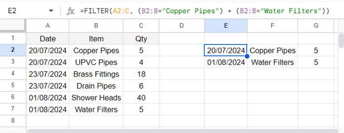
=FILTER(A2:C, (B2:B="Copper Pipes") + (B2:B="Water Filters"))This will apply multiple conditions to filter the same column, where the column is filtered for the criteria “Copper Pipes” and “Water Filters.”

Multi-Condition Filtering in the Same Column Using Criteria from a Range
We usually specify criteria in a range and refer to that in the formula when dealing with multiple criteria.
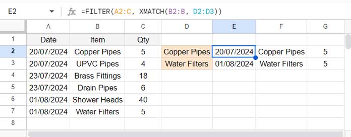
For example, if you want to filter a range for items “Copper Pipes” and “Water Filters” in column B, you can enter these criteria into two cells—say, “Copper Pipes” in cell D2 and “Water Filters” in cell D3—and use the formula:
=FILTER(A2:C, (B2:B=D2) + (B2:B=D3))This approach works, but it’s not ideal for a large number of criteria. Instead, you can match a criteria range (e.g., D2:D3) against column B using the XMATCH function, like this:
=FILTER(A2:C, XMATCH(B2:B, D2:D3))
In this formula, XMATCH follows the syntax:
XMATCH(search_key, lookup_range, [match_mode], [search_mode])- where
search_keyis the range to be matched (B2:B) andlookup_rangeis the range containing the criteria (D2:D3).
XMATCH returns the relative position of each item in search_key within lookup_range if a match is found, otherwise, it returns #N/A.
The FILTER function returns rows where the condition is a number, meaning that XMATCH found a match.
Resources
- Comma-Separated Values as Criteria in Filter Function in Google Sheets
- Filter Based on a List in Another Tab in Google Sheets
- Filter Data by Date Range in Google Sheets
- Filter Out Matching Keywords in Google Sheets – Partial or Full Match
- Filter Rows Based on Criteria List with Wildcards in Google Sheets
- How to Filter Next Row to the Filter Criteria Row in Google Sheets
- How to Hardcode DATETIME Criteria within FILTER Function in Google Sheets
- How to Use AND and OR with the Google Sheets FILTER Function
- How to Use Date Criteria in the FILTER Function in Google Sheets


=FILTER(Data!$A:$AN,Data!$P:$P ="",Data!$E:$E ="",Data!$U:$U ="",(Data!$G:$G "Deal Cancelled")+(Data!$G:$G ""&"")+(Data!$G:$G""&"Buyback"))Error Occurred anyone helps me to get resolved this formula.
Hi, Arvind Kumar,
You may please try either of the below Filter or Query formulas.
Filter;
=FILTER(Data!$A:$AN,Data!$P:$P ="",Data!$E:$E ="",Data!$U:$U ="",(Data!$G:$G= "Deal Cancelled")+(Data!$G:$G="")+(Data!$G:$G="Buyback"))Query;
=QUERY(Data!$A:$AN,"Select * where P is null and E is null and U is null and (G= 'Deal Cancelled' or G is null or G='Buyback')")If this is not working, please explain the problem instead of giving a non-working formula.
Thanks.
Thanks, this was really helpfull!