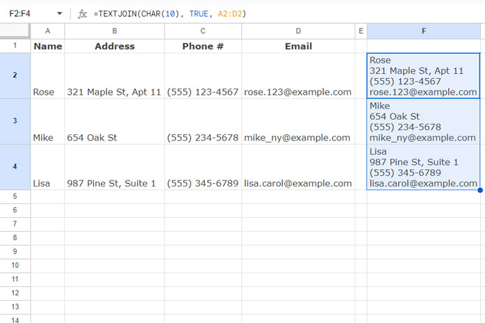
This tutorial is not about combining values across multiple columns but rather about placing multiple column values into a single cell as new lines in Google Sheets.
When could this be useful in real life?
Suppose you have a spreadsheet where employee addresses are entered in multiple columns, like this:
Table # 1:
| Name | Address | Phone # | |
| Rose | 321 Maple St, Apt 11 | (555) 123-4567 | rose.123@example.com |
You may want to combine these column values into a single cell with each value on a new line for printing labels or other purposes.
Table # 2:
| Rose 321 Maple St, Apt 11 (555) 123-4567 rose.123@example.com |
In such cases, instead of manually copying and pasting, which is time-consuming, you can use the following formula to automate the process.
Multiple Columns into a Multi-Line Single Cell: Non-Array Formula
My sample data spans across A1:D, with A1:D1 containing the column names Name, Address, Phone #, and Email.

To combine the information from multiple columns into a single cell with each value on a new line, you can use the TEXTJOIN function as follows:
In cell F2, enter the following formula and drag it down as needed:
=TEXTJOIN(CHAR(10), TRUE, A2:D2)Explanation:
TEXTJOIN(delimiter, ignore_empty, text1, [text2, …])delimiter(the separator between each cell value) isCHAR(10), which represents a new line character.ignore_emptyis set toTRUE, which removes empty cells while combining.text1is the rangeA2:D2.
This formula combines the values in A2:D2 into a single cell with each value on a new line. When you drag the formula down, it applies to the data in the corresponding rows.
Multiple Columns into a Multi-Line Single Cell: Array Formula
If you prefer using Array Formulas, you might have tried the following formulas in cell F2:
=TEXTJOIN(CHAR(10), TRUE, A2:D)And:
=ArrayFormula(TEXTJOIN(CHAR(10), TRUE, A2:D))Unfortunately, both formulas will return the same result and might not meet your needs.
To handle multiple column values in a single cell across multiple rows, use the following array formula in cell F1:
=ArrayFormula(
   TRIM(
      TRANSPOSE(
         SPLIT(
            TEXTJOIN(CHAR(10), TRUE, {"~"&A2:A, B2:D}), "~"
         )
      )
   )
)
Explanation:
TEXTJOIN(CHAR(10), TRUE, {"~"&A2:A, B2:D})combines the values from multiple columns into a single text string, with each value separated by a new line (CHAR(10)), and adds a~before the values in the first column.- To test this, use a closed range and include the ARRAYFORMULA as follows:
=ArrayFormula(TEXTJOIN(CHAR(10), TRUE, {"~"&A2:A4, B2:D4}))
Result:
| ~Rose 321 Maple St, Apt 11 (555) 123-4567 rose.123@example.com ~Mike 654 Oak St (555) 234-5678 mike_ny@example.com ~Lisa 987 Pine St, Suite 1 (555) 345-6789 lisa.carol@example.com |
SPLIT(…, "~")splits the combined text string based on the~delimiter, placing each address across the row.
| Rose 321 Maple St, Apt 11 (555) 123-4567 rose.123@example.com | Mike 654 Oak St (555) 234-5678 mike_ny@example.com | Lisa 987 Pine St, Suite 1 (555) 345-6789 lisa.carol@example.com |
TRANSPOSE(…)arranges the split results into a vertical format.- The TRIM function removes any extra blank lines introduced during the process.
Lambda Approach
You can use the BYROW lambda function to simplify the drag-down TEXTJOIN formula.
Instead of using the regular array formula, you can use the following BYROW formula in cell F2 to combine multiple column values into a single cell in Google Sheets:
=BYROW(A2:D, LAMBDA(row, TEXTJOIN(CHAR(10), TRUE, row)))Explanation:
- The BYROW formula processes each row in the array A2:D and applies the TEXTJOIN function to combine the values in that row into a single cell, separated by newlines (
CHAR(10)). - The
rowin the LAMBDA function represents each row of data from the array A2:D.
You can use any of the above formulas to combine multiple column values into a single cell. However, I recommend avoiding the LAMBDA approach if you have a large dataset, as it may impact performance.
Resources
- How to Move New Lines in a Cell to Columns in Google Sheets
- Start New Lines Within a Cell in Google Sheets
- Extract Every Nth Line from Multi-Line Cells in Google Sheets
- How to Match | Extract Nth Word in a Line in Google Sheets
- Remove Whitespaces at the Beginning of a Newline in Google Sheets
- Finding Duplicates in New Lines Inside Cells in Google Sheets
- Sorting Data Separated by Line Breaks within Google Sheets Cells


Prashanth, Excellent contribution. An error appears.
“Error In ARRAY_LITERAL, an Array Literal was missing values for one or more rows.”
I am in the dark 🙁 Could you please share a sample?
Hi Prashanth, how do I share the spreadsheet?
Waiting for ‘access’!
Hi, Harvi,
Corrected the formula on your sheet. It, I mean the error, was due to regional (Locale) settings. Please read this.
How to Change a Non-Regional Google Sheets Formula
Thank you very much!