


")


")

")
")
 in Excel & Google Sheets")


There are three main formula approaches to move values from alternate rows to columns in Google Sheets, and all of them can handle multiple columns simultaneously. Below, we’ll explore each approach in detail, using an example dataset.
Sample Data Setup
Assume you have the following sample data in columns A and B:
| Project Phase | Date |
| Project Start | 2024-11-01 |
| Project End | 2024-11-20 |
| Project Start | 2024-11-16 |
| Project End | 2024-11-14 |
| Project Start | 2024-11-20 |
| Project End | 2024-11-28 |
| Project Start | 2024-11-28 |
| Project End | 2024-11-30 |
In this example, the data in columns A and B alternates between project start and project end dates. You want to move the “Project Start” rows into one column and the “Project End” rows into another column.
We will be working with the range A2:B (assuming the headers are in row 1). You can apply these formulas to either both columns or just one column depending on your need.
Option 1: Using the FILTER Function to Move Alternate Rows to Columns
The FILTER function allows you to filter a range based on a condition. You can use it to filter and move alternate rows into columns.
Formula:
=FILTER(A2:B, ISODD(SEQUENCE(ROWS(A2:A))))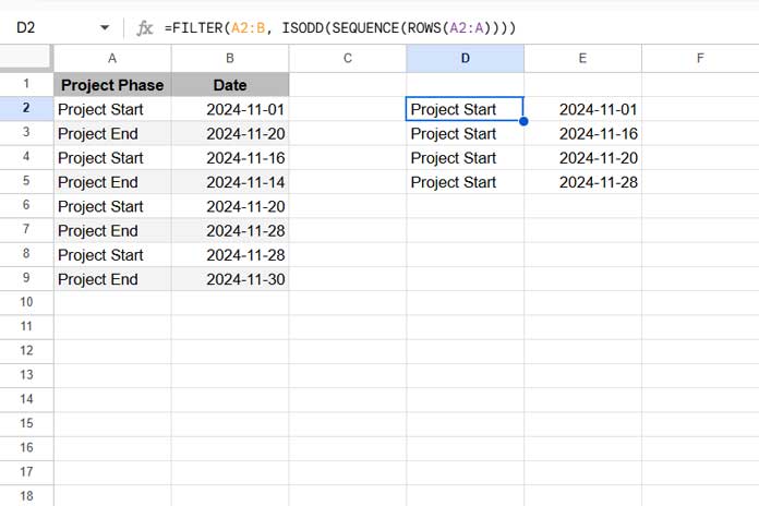
Explanation:
SEQUENCE(ROWS(A2:A)): This generates a sequence of numbers equal to the number of rows in the rangeA2:A. For example, if there are 8 rows, the sequence would be{1, 2, 3, 4, 5, 6, 7, 8}.ISODD(SEQUENCE(...)): This checks if the sequence numbers are odd, and if so, it returnsTRUEfor every odd-numbered row (i.e., rows 1, 3, 5, etc.).
This formula will move both columns (“Project Start” and “Date”) from alternate rows. To move data from only the first column (e.g., “Project Start”), replace the filter range A2:B with A2:A.
For the “Project End” values, you can replace ISODD with ISEVEN to capture every alternate row starting from the second row:
=FILTER(A2:B, ISEVEN(SEQUENCE(ROWS(A2:A))))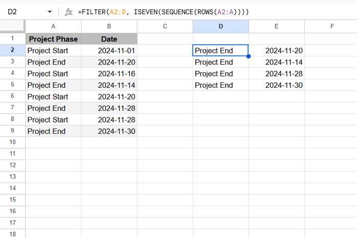
Option 2: Using the QUERY Function to Move Data from Alternate Rows to Columns
While the QUERY function does not officially support a “skipping” clause, it works effectively with certain syntax to return alternate rows.
Formula:
=QUERY(A2:B, "SELECT * SKIPPING 2")Explanation:
SKIPPING 2: This instructs the QUERY function to skip 2 rows starting from the current row (inclusive), effectively returning every other row.
You can adjust the range to move data from a single column. For example, use A2:A to pull data from only the “Project Start” column.
To move every second, fourth, sixth row, change the range to A3:B:
=QUERY(A3:B, "SELECT * SKIPPING 2")Option 3: Using CHOOSEROWS to Move Data from Alternate Rows to Columns
The CHOOSEROWS function allows you to specify which rows to include in a result. This can be particularly useful when you want to move alternate rows into columns.
Formula:
=CHOOSEROWS(A2:B, SEQUENCE(ROWS(A2:A)/2, 1, 1, 2))Explanation:
SEQUENCE(ROWS(A2:A)/2, 1, 1, 2): This generates a sequence of row numbers, starting from 1, with a step of 2 (i.e., 1, 3, 5, 7, etc.). This sequence will return every odd-numbered row in the range.ROWS(A2:A)/2: This determines how many rows should be included, based on the total number of rows in the rangeA2:A.
To capture data from even-numbered rows (i.e., the second, fourth, sixth rows), use:
=CHOOSEROWS(A2:B, SEQUENCE(ROWS(A2:A)/2, 1, 2, 2))Conclusion
These three formulas provide different ways to move alternate rows into columns in Google Sheets. Whether you use FILTER, QUERY, or CHOOSEROWS, you can manipulate your data in a flexible and efficient way. Choose the formula that best fits your needs depending on the specific data and requirements.
What if you have a list and you want to auto deposit it into another column – but skipping every 4th entry? So I have a list in Column A and want to transfer it to Column B but with a blank cell in between each row. Almost as if it was the reverse of
=query(A:A, "select A skipping 2")A quick response would be greatly greatly appreciated. Thank you very much!
Hi, Jacob Noble
This is the reverse of the above-said Query plus a blank row in between.
=ArrayFormula(if(IFERROR(if(len(A1:A),mod(row(A1:A),2),))=0,A1:A,))