In this quick tutorial, I’ll elaborate on the use of the statistical function MODE.MULT in Google Sheets.
To find the mode value, you can use the MODE function. The mode value represents the most common number in a dataset.
However, what is the significance of the MODE.MULT function if there’s already a MODE function available in Google Sheets?
In this post, I’ll delve into the role of the Google Sheets MODE.MULT function and provide some additional tips.
MODE.MULT Function: Syntax and Formula Examples in Google Sheets
Syntax:
MODE.MULT(value1, [value2], ...)Arguments:
value1: The first value or range to consider.[value2], …: Optional. Additional values or ranges to consider.
When specifying ranges in value1, value2, etc., they can be of the same size or different sizes, such as =MODE.MULT(A1:A10, C1:C10) or =MODE.MULT(A1:A10, C10:C25).
Basic Examples
=MODE.MULT(5, 4, 5, 2)The above MODE.MULT formula would return #5 as the mode value (the most frequently occurring number).
The following MODE formula would also produce the same output:
=MODE(5, 4, 5, 2)The distinction between MODE and MODE.MULT lies in the latter’s ability to return multiple modes. We will explore this in the example below.
MODE.MULT: The Multiple Mode Function
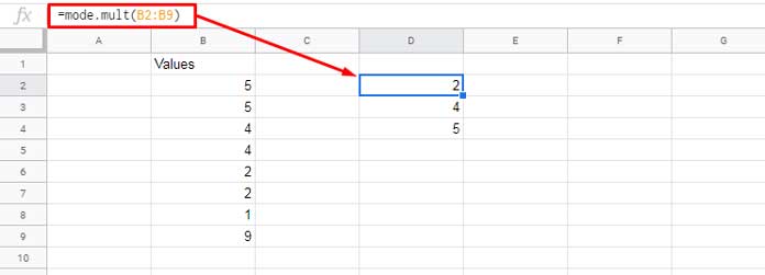
Assuming you have a dataset in the range B2:B9 with multiple model numbers, the MODE function alone won’t suffice. To return multiple modes, you must use the MODE.MULT function.
=MODE.MULT(B2:B9)The formula returns the numbers 2, 4, and 5 as the range contains {5; 5; 4; 4; 2; 2; 1; 9}. The output is sorted in ascending order by default.

If you use MODE, it will only return the first mode, which in our example would be #5.
Key Points:
- When using the MODE.MULT function, ensure there are enough blank cells below the formula’s application cell. Otherwise, the formula may sometimes return a #REF error.
- The MODE.MULT function is an array formula. Unlike Excel versions that only support legacy array formulas, you don’t need to enter this formula as an array formula by pressing Ctrl+Shift+Enter or using the ARRAYFORMULA function in Google Sheets.
- If no values occur more than once, the function returns a #N/A error.
- The function ignores text and blank cells in the range.
- If error values are present in the range, the formula will return an error. To remove error values, you can use TOCOL if the range is vertical and TOROW if the range is horizontal. For example:
=MODE.MULT(TOCOL(D8:D13, 3)).
How to Check for Multiple Modes in a Range
To test whether a dataset contains multiple model numbers, you can use the IF and COUNT functions with the MODE.MULT function as shown below:
=IF(COUNT(MODE.MULT(B2:B9))>1,"Multiple Modes","")Explanation:
MODE.MULT(B2:B9): Returns the modes in the range.COUNT(…): Returns the count of values in the MODE.MULT result.
The logical expression in the IF function is COUNT(MODE.MULT(B2:B9))>1. If true, the formula returns “Multiple Modes”; otherwise, it returns an empty result. This follows the syntax IF(logical_expression, value_if_true, value_if_false).
With this example, we conclude this tutorial. Thank you for your attention, and we hope you found it helpful!


