 in Google Sheets")

")

")


")


")


, N(), T(), and DATEVALUE().)
To solve or handle the Mixed Data Type Issue in Query in Google Sheets, you can use functions like TO_TEXT, N, T, DATEVALUE, and info-type functions based on the situation.
In this tutorial, I’ll focus on the formula-based solutions, which are crucial to understand.
What is a Mixed Data Type in Query?
A mixed data type column occurs when a single column in your dataset contains both text and numbers or other mixed types. Examples:
- Text & Numbers
- Text & Dates
- Text & Boolean (TRUE/FALSE)
- Numbers & Dates
How Does Mixed Data Affect Query?
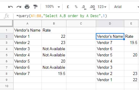
When running a Query in Google Sheets, the function determines the column’s data type based on the majority of its values. The minority data types are treated as null (missing values) in the output.
For example, let’s say column B contains a mix of numbers and text:
=QUERY(A1:B8, "SELECT A, B ORDER BY A DESC", 1)This might cause text values in column B to disappear in the Query results because numbers dominate the column.
Let’s look at ways to fix this issue.
1. Convert Numbers to Text Using TO_TEXT in Query
A popular solution among Google Sheets users is TO_TEXT, which ensures all values in a column are treated as text.
Formula:
=ArrayFormula(QUERY({A2:A8, TO_TEXT(B2:B8)}, "SELECT Col1, Col2 ORDER BY Col1 DESC", 0))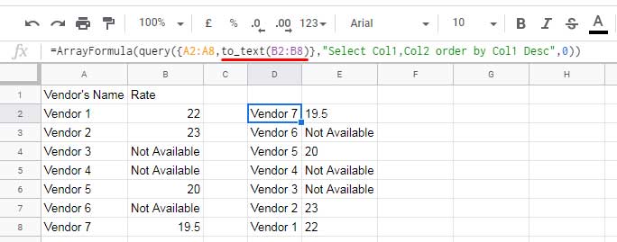
How It Works:
- We create a virtual dataset (
{A2:A8, TO_TEXT(B2:B8)}) where column B is entirely text. - We refer to columns as
Col1andCol2instead ofAandB. - ArrayFormula is used since TO_TEXT is not an array function by default.
Drawback:
Numbers in column B are now text, so calculations within Query may not work correctly. If calculations are required, use the N function instead.
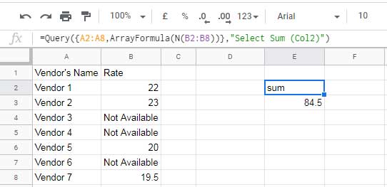
2. Retain Numbers & Convert Text to 0 Using N in Query
Instead of TO_TEXT, we can use N, which:
- Retains numbers as they are.
- Converts text values to 0.
Formula:
=ArrayFormula(QUERY({A2:A8, N(B2:B8)}, "SELECT SUM(Col2)"))Use Case:
If you want to perform calculations (e.g., SUM()) on column B, N ensures numbers remain usable while converting non-numeric values to 0.
3. Convert Numbers to Null & Keep Text Using T in Query
If your priority is keeping text and ignoring numbers, use the T function, which:
- Retains text as it is.
- Converts numbers to null (empty values).
Formula:
=ArrayFormula(QUERY({A2:A8, T(B2:B8)}, "SELECT *"))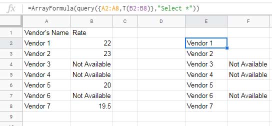
This ensures that only text values from column B appear in the Query output.
4. Handle Mixed Text & Numbers Using Info Functions
You can use info-type functions like ISNUMBER and ISTEXT within IF statements to structure data in a way that Query can process correctly.
Convert a Text & Number Column to Numbers:
=ArrayFormula(QUERY({A2:A8, IF(ISNUMBER(B2:B8), B2:B8, 0)}, "SELECT *", 0))- Numbers remain unchanged
- Text values are replaced with
0
Convert a Text & Number Column to Text:
=ArrayFormula(QUERY({A2:A8, IF(ISTEXT(B2:B8), B2:B8, "")}, "SELECT *", 0))- Texts values remain unchanged
- Numbers are converted to
""(empty strings), effectively making the column text-only
5. Handling Mixed Date & Text or Date & Number Columns Using DATEVALUE in Query
If your column contains both dates and text, use DATEVALUE instead of ISDATE, since ISDATE does not return an array result.
Formula (Extract Dates Only):
=ArrayFormula(QUERY({A2:A8, TO_DATE(DATEVALUE(B2:B8))}, "SELECT *", 0))- Extracts date values while ignoring text values.
- TO_DATE ensures that valid dates display correctly in the Query output.
Note: If the column contains both numbers and dates, the formula extracts only dates.
Formula (Extract Numbers Only, Ignoring Dates):
If your column contains both dates and numbers and you want to return only numbers, use:
=ArrayFormula(QUERY({A2:A8, IF(NOT(IFERROR(DATEVALUE(B2:B8))), B2:B8, "")}, "SELECT *", 0))- Extracts numbers while ignoring dates
Why Create Virtual Columns?
We use virtual columns ({A2:A8, TO_TEXT(B2:B8)}) to bypass Google Sheets Query’s default behavior, where the majority data type dictates column type. This allows us to force Query to process all values correctly.
Conclusion
- If you need all values as text, use
TO_TEXT. - If you need calculations on numeric values, use
N. - If you need only text, use
T. - If working with mixed date & text or date & number columns, use
DATEVALUE(). - Use info functions (
ISNUMBER,ISTEXT) for more control over data type conversion.
By using these workarounds, you can prevent missing values and ensure Query processes your data correctly.
How will I place the curly bracket if it’s Query and Importrange?
E.g:
=query({IMPORTRANGE(C1,"Staff!A3:V");IMPORTRANGE(C1,"Staff_ATT!A3:V")},
"select * where Col2 is not null",0)
My column A is supposed to be all Numbers. However, whenever I consolidate them in one Sheet, it returns only blank.
So I want to ensure that all datatype are either numbers or text.
Hi, Paulo,
In that case, use FILTER.
You may please try this one.
=LET(data,VSTACK(IMPORTRANGE(C1,"Staff!A3:V"),IMPORTRANGE(C1,"Staff_ATT!A3:V")),
filter(data,len(choosecols(data,2))))
You can check my Function Guide to learn the new functions used above, such as LET, VSTACK, and CHOOSECOLS.
Thank you very much for this article.
I didn’t understand why some values were disappearing, and you explained it perfectly.
I wanted to append the results of several QUERY functions and so wrapped the whole combination with another QUERY.
One of the columns has a mixed type, i.e., boolean and text and the values were disappearing.
What I did is I split the big long query into two parts (one for the booleans and one for the text).
I didn’t use to_text at all.
Hi, Karim,
Thanks for your feeback!
Works like wonder! Thanks, Prashant, would love to understand how this works if you could point me to the relevant post for an explanation, thanks again.
Hi Prashant,
I’ve been reading a number of your posts trying to figure out how to solve this, looks like I still need your advice. I need to extract a Date and Time from 2 columns and merge them into one column, at the same time still keeping them in Number format. After joining them I had a problem turning them back to Number again as I need it later to identify the month, date, etc.
Attaching the “MD” sheet here for reference, cells in orange. Thank You, Prashant
Hi, Junnie Chen,
Inserted the below formula in MD!G1.
={"Date";ArrayFormula(if(len('Form Responses 2'!T2:T),'Form Responses 2'!T2:T+'Form Responses 2'!U2:U,))}Column formatted to Date Time (Format > Number > Date Time)
Your last formula in the TO_TEXT-part looks like this:
=ArrayFormula({A1:B1;query({A2:A8,to_text(B2:B8)},"Select Col1,Col2 order by Col1 Desc",0)})I assume, that the written semicolon should be a comma for an English expression. (For German expressions we use semicolons in functions, outside of SELECT-statements.)
Hi, Joe76,
Nope! It should be a semi-colon as it’s the header row.
You may like: How to Change a Non-Regional Google Sheets Formula.
Thank you !!! You saved me a lot of time explaining query mixed data problem in a complete article like this.