I prefer to use array formulas whenever possible to complete tasks in Google Sheets. I have an array formula to offer for finding missing sequential dates or numbers in a list in Google Sheets.
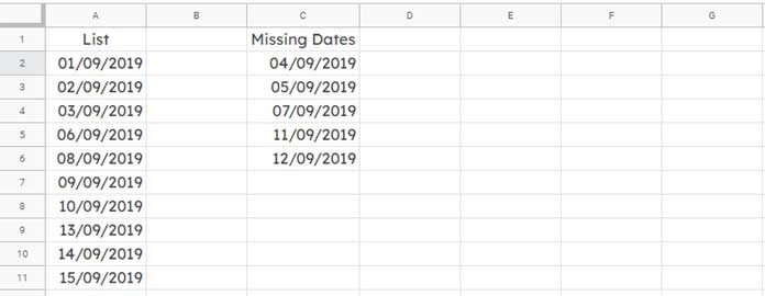
For example, let’s say you have a list of dates in column A in Google Sheets. You want to find the missing dates in this list, regardless of whether the dates are ordered in sequential order or not.
In the following example, column A contains the list, and column C contains the missing dates that are returned using an array formula in cell C2.
Example of finding missing sequential dates in a list in Google Sheets:

How to Find Missing Sequential Dates in Google Sheets
Syntax:
LET(name1, value_expression1, [name2, …], [value_expression2, …], formula_expression)Here is the array formula I used in cell C2 to list the missing sequential dates.
Master Formula:
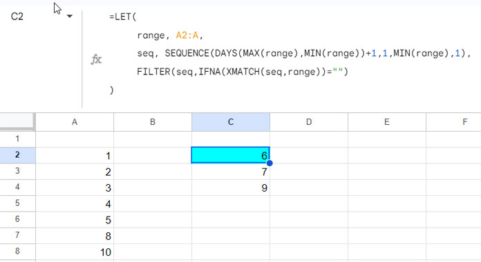
=LET(
     range, A2:A,
     seq, SEQUENCE(DAYS(MAX(range),MIN(range))+1,1,MIN(range),1),
     FILTER(seq,IFNA(XMATCH(seq,range))="")
)
Where:
range: The range of cells that contains the list of dates.seq: The list of all possible dates between the first and last dates in the range.formula_expression: The formula that filters (extracts) the missing dates from the list of possible dates.
You just specify the range containing the list (here, it is A2:A). The formula will take care of the rest.
This is an array formula, so it will cover all the dates in the list in column A and then populate the missing sequential dates in column C.
You can simply enter the array formula in cell C2. You do not need to copy and paste the formula to the cells below. However, make sure that the cell range C2:C is blank before entering the formula.
Formula Explanation
The range is A2:A, so it does not require any further explanation. Let’s see the seq and formula_expression parts in detail below.
I have used eight native Google Sheets functions in the above formula. They are;
- DAYS, MIN, and MAX
- SEQUENCE
- LET
- XMATCH, IFNA, and FILTER
I will try to explain the role of each one of them in a clear-cut manner in populating missing sequential dates in Google Sheets.
Generating Sequential Dates Based on Start and End Dates in the List: seq Part
We can use the following SEQUENCE formula (seq) to generate a list of sequential dates from 01/09/2019 (the minimum date in the range) to 15/09/2019 (the maximum date in the range).
SEQUENCE(DAYS(MAX(range),MIN(range))+1,1,MIN(range),1)Expanded Form:
=SEQUENCE(DAYS(MAX(A2:A),MIN(A2:A))+1,1,MIN(A2:A),1)Syntax:
SEQUENCE(rows, [columns], [start], [step])Explanation:
- The
rowsargument specifies the number of values to return. This number is equal to the number of days between the minimum and maximum dates in A2:A. TheDAYS(MAX(A2:A),MIN(A2:A))+1formula returns that number. - The
columnsargument is optional. We set it to 1 because we want the sequential dates to be in one column. - The
startargument specifies the starting value. In this case, we want to start with the minimum date in the range A2:A. - The
stepargument is optional. We set it to 1 because we want the dates to be increased by 1.
We should now compare this sequence to the range A2:A. Then, we can extract the mismatching values. Those will be the missing sequential dates in the list (range).
Filter Missing Sequential Dates Comparing Two Lists: formula_expression Part
The following FILTER formula (formula_expression) filters missing sequential dates by comparing two lists.
FILTER(seq,IFNA(XMATCH(seq,range))="")Formula_Expression in Expanded Form (replaced seq with the corresponding formula and range with A2:A):
=FILTER(SEQUENCE(DAYS(MAX(A2:A),MIN(A2:A))+1,1,MIN(A2:A),1),IFNA(XMATCH(SEQUENCE(DAYS(MAX(A2:A),MIN(A2:A))+1,1,MIN(A2:A),1),A2:A))="")Let’s explain this formula in more detail.
We have compared two lists in the formula. List 1 (seq) is the sequence of numbers generated by the SEQUENCE function in the previous step. List 2 (range) is the dates in the range A2:A.
For comparison, we use the XMATCH function.
Formula:
XMATCH(seq,range)Syntax:
XMATCH(search_key, lookup_range, [match_mode], [search_mode])In this formula, the search_key is the sequence of dates (seq) and the lookup_range is the dates in A2:A.
This will return a #N/A value if the date in the sequence is not found in the range A2:A.
We use the IFNA function to replace #N/A with a blank value.
IFNA(XMATCH(seq,range))The FILTER formula filters the sequence of dates if the IFNA + XMATCH combination is equal to blank.
This way, we can find missing sequential dates in a list in Google Sheets.
The formula will also work with a list of numbers. Please try it yourself.

Resources:


Hi Prashanth, thank you for your work.
This formula works well for me.
Is there a similar formula that can count the number of sequences of four consecutive working days between two dates?
Thank you.
Hi Yann,
I assume weekends (Sat/Sun) break the consecutiveness. There are two ways to approach this problem—one is to expand the date range with SEQUENCE() and count each possible 4-day stretch, and the other is to use a direct formula approach. I went with the latter, since the first method can be resource-intensive for large ranges.
You can try my formula below (replace A1 and B1 with your respective start and end dates):
=LET(start, A1, end, B1, wdS, WEEKDAY(start, 2), x, IF(LTE(wdS, 2), start-wdS+2, start-wdS+9), wdE, WEEKDAY(end, 2), y, IF(OR(wdE=4, wdE=5), end-wdE+5, IF(GT(wdE, 5), end-wdE+6, end-wdE-2)), MAX(0, INT(NETWORKDAYS(x, y)/4))*(GT(NETWORKDAYS(start, end), 3)))I have updated this post with a new formula!
Hi, Prashanth
Can you help me with this? I tried following your method to a set of two columns with one column missing some dates.
I am unable to sort it. I just want the column to appear blank where the dates are missing.
Sure, feel free to email me a copy of the mockup sheet or post the URL below.
I tried this formula but not working.
Hi, Ashok Kumar,
I’ve replied to your email. Please check.
Hi, Ashok Kumar,
Thanks for sharing your Spreadsheet.
The above formula works for me! Please check the “Test” tab in your sheet.
Thank you. It all works. The only problem I have is my list of dates keeps growing, and I need to find the dates that are not included as the list grows. So my formula needs to include blanks where the dates will drop in. So in the example, you provided, I extended A11 to say A40 (where A12 to A40 are blanks anticipating date entry) but got an error. Can you help?
Hi, John,
You can use MAX and MIN as below.
Replace cell references/cell range as detailed below.
Replace all
A11withmax(A2:A),A2:A11withA2:A, and A2 withmin(A2:A)Example formula for cell range A2:A
=Filter(sequence(max(A2:A)-min(A2:A)+1,1,min(A2:A),1),Regexmatch(to_text(to_date(sequence(max(A2:A)-min(A2:A)+1,1,min(A2:A),1))),textjoin("|",1,A2:A))=FALSE)In some cases, the formula won’t return the correct result. It may be matching issues due to date formatting.
The preferred date formatting is dd/mm/yyyy or mm/dd/yyyy depending on your sheets settings.
Thank you, Prashanth, for this tutorial in the body of this post and also for the use of MAX and MIN for a set of entries that will grow.
Hi,
How can we use the formula in listing all working dates between two dates? (Mon-Fri are Network days).
Also, is it possible to list the next 5 working dates from a Start Date?
I appreciate the help!
Hi, Zatin,
To list the next 5 working days use the following array formula.
C2 contains the start date. You can use
=today()in C2 to get next 5 working days.=ArrayFormula(WORKDAY.INTL(C2,sequence(5,1),1))This has already explained – How to Populate Sequential Dates Excluding Weekends in Google Sheets.
Regarding the same with an end date specified, I’ll write the tutorial soon and let you know.
Best,
https://infoinspired.com/google-docs/spreadsheet/working-dates-between-two-dates-in-google-sheets/
Hi there!!
I have tried to make the formula work but it doesn’t, well… it does, partially.
I don’t know why it fails.
Sample Sheet, please…