Find the Longest String in a Column in Google Sheets

This post introduces four formula options to find the Longest String in a Column in Google Sheets. You can choose the formula based on your requirement. Out of the four, three formulas return a single longest text in a column, but if there are multiple longest strings, you should use the fourth one to get all of them.

Finding the Longest String in a Column in Google Sheets is all about identifying strings based on the maximum number of characters. So, the backbone of the formulas is the LEN function, which returns the length of the text.

Purpose

The purpose may vary from user to user. For me, it’s quite useful in certain scenarios. For example, if you’re analyzing survey results, reviews, or descriptions, finding the longest response might help spot detailed or verbose entries worth special attention.

Find the First String with the Longest Length

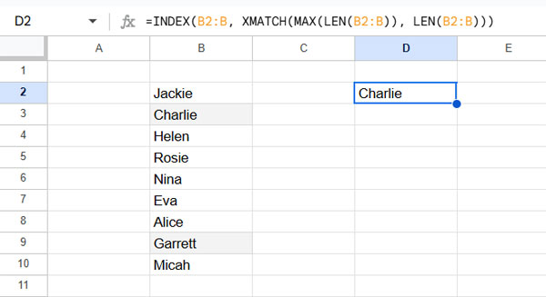
Assume you have a list of names in column B, range B2:B, as follows:

Jackie
Charlie
Helen
Rosie
Nina
Eva
Alice
Garrett
Micah

You can find the name with the most number of characters with the following formula.

Remember! If there is a tie in the number of characters, the formulas will return the first longest string — meaning the first name found.

Formula 1:

=INDEX(B2:B, XMATCH(MAX(LEN(B2:B)), LEN(B2:B)))

This formula returns “Charlie,” which is the longest string in column B.

Example of Finding the First String with the Longest Length

Actually, there is one more name with the same number of characters, “Garrett.” Since “Charlie” appears first, the formula returns it.

LEN returns the length of characters in each name.
XMATCH finds the position of the first occurrence of the maximum length.
INDEX uses that position to return the corresponding name.

Formula 2:

=ARRAYFORMULA(XLOOKUP(MAX(LEN(B2:B)), LEN(B2:B), B2:B))

This will also return “Charlie.”

LEN returns the length of characters in each name.
XLOOKUP searches for the maximum length in the array and returns the first match.
ARRAYFORMULA ensures LEN processes the full range as an array. In the earlier formula, INDEX handled array behavior naturally.

Formula 3:

Here is the third formula to find the Longest String in a Column in Google Sheets:

=CHOOSEROWS(SORT(B2:B, LEN(B2:B), 0), 1)

This will also return “Charlie.”

SORT sorts the names in descending order by their length.
CHOOSEROWS extracts the first name from the sorted list.

Find All Strings with the Longest Length

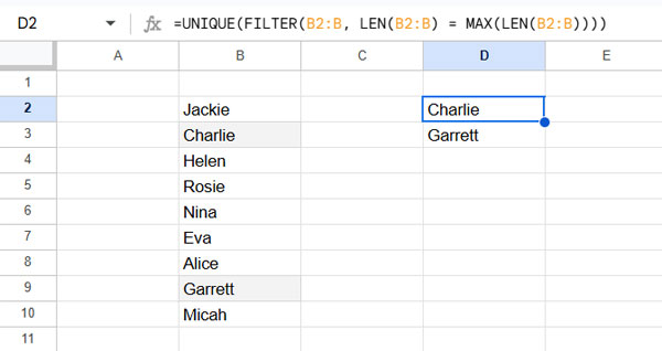
As you go through the sample names, you can see that the longest strings are “Charlie” and “Garrett,” both with the same number of characters. All the above formulas return only the first occurrence.

To find all strings with the longest length — meaning every string tied for the maximum length — you can use the formula below.

=UNIQUE(FILTER(B2:B, LEN(B2:B) = MAX(LEN(B2:B))))

FILTER returns the names in B2:B where the length equals the maximum length.
UNIQUE removes duplicates, if any.

Example of Finding All Strings with the Longest Length

This way, you can find all the strings tied for the Longest String in a Column in Google Sheets.

FAQ: Find the Longest String in a Column in Google Sheets

What if multiple entries have the same longest length?

If multiple strings have the same maximum number of characters, most formulas in this post will return only the first occurrence. To find all entries tied for the longest length, use the FILTER + UNIQUE formula shared above.

Can I find the longest string across multiple columns?

Yes! Instead of referencing a single column like B2:B, you can reference a range across multiple columns, like B2:D.

To do this, replace every instance of B2:B with col inside the formula, and plug that formula into the structure below:

=BYCOL(B2:C, LAMBDA(col, formula_here))

Example:

To find all longest strings in each column separately:

=BYCOL(B2:D, LAMBDA(col, CHOOSEROWS(SORT(col, LEN(col), 0), 1)))

This formula will return the longest string(s) from each column individually.

What happens if the column contains blank cells?

Blank cells have a length of zero, so they won’t affect the results when finding the Longest String in a Column in Google Sheets. The formulas will simply ignore blanks.

How do I highlight the longest string instead of returning it?

You can use Conditional Formatting with a custom formula like:

=LEN(B2) = ARRAYFORMULA(MAX(LEN($B$2:$B)))

This will highlight all cells in the column that match the longest length.

Does this method work with numbers too?

Technically yes — numbers will be treated as text if necessary. However, if you want to specifically target numbers, you may need to wrap the range with TO_TEXT to ensure consistent behavior.

How to Find the Longest String in a Column in Google Sheets