


")


")

")
")
 in Excel & Google Sheets")


Checkboxes, also known as tick boxes, have many uses in Google Sheets. Dependent checkboxes are my favorite so far, but here’s another great tip: you can lock and unlock cells using checkboxes in Google Sheets.
How It Works
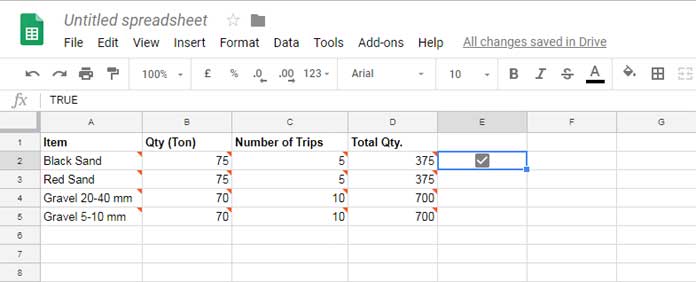
Imagine you want to lock cells in each row and control them with checkboxes. For example, you want to lock/unlock the cells in the range A2:D2 by toggling the checkbox in cell E2.
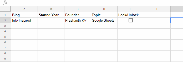
- When you check the checkbox, the cells lock.
- When you uncheck it, the cells unlock for editing.
This helps prevent accidental edits to specific rows.
Lock and Unlock Cells Using Checkboxes in Google Sheets
You can control the locking and unlocking of cells in two ways:
- Using multiple checkboxes, each controlling a row.
- Using a single checkbox to lock/unlock an entire range.
Let’s explore both methods.
1. Lock and Unlock Cells Using Multiple Checkboxes
Follow these steps to configure the cells and checkboxes:
Steps:
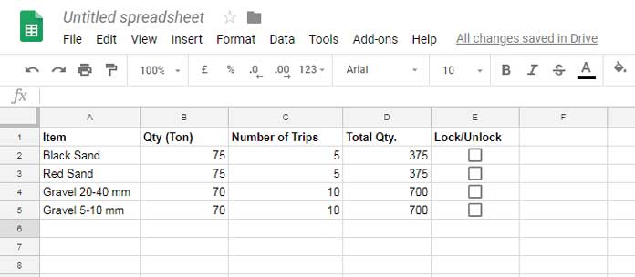
- Insert checkboxes in the range E2:E5.
- Select E2:E5.
- Go to Insert > Tick Box.
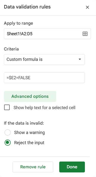
- Select the range A2:D5 (the cells to be locked/unlocked based on the checkboxes).
- Go to Data > Data validation.
- Click on + Add rule.
- Under Criteria, select Custom formula is.
- Enter the following formula:
=$E2=FALSE - Under Advanced settings, select Reject input.
- Click Done.
Now, when you check a checkbox, the corresponding row will be locked. You won’t be able to edit any content in that row unless you uncheck the box.
For example, if you check the box in E3, the cells in A3:D3 will be locked. To edit them, you must uncheck the box in E3.
Restrict Checkbox Deletion (Additional Layer of Protection)
If you’re the only one using the sheet, this may not be necessary. However, if you share it with others who have editing rights, they may accidentally override the protection.
For instance, they could uncheck all checkboxes and edit the cells or even delete entire rows or columns. To prevent this:
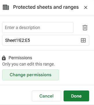
- Select E2:E5 (the checkboxes).
- Right-click the sheet tab and select Protect sheet.
- In the sidebar, click Range > Set permissions.
- Under Restrict who can edit this range, select Only you.
- Click Done.
Now, users can edit only the rows where the checkbox is unchecked. They cannot delete the checkboxes or the rows containing them.
To prevent them from deleting columns in the protected range, protect the header row (A1:D1) using the same method:
- Repeat steps 1 to 5, but in step 1, select A1:D1 instead of E2:E5.
2. Lock and Unlock Cells Using a Single Checkbox
You can control an entire range of cells with a single checkbox. Here, the checkbox is in cell E2, and it locks/unlocks the range A2:D5.
Steps:
- Insert a checkbox in E2.
- Select the range A2:D5.
- Go to Data > Data validation.
- Click + Add rule.
- Under Criteria, select Custom formula is.
- Enter the following formula:
=$E$1=FALSE - Under Advanced settings, select Reject input.
- Click Done.
Now, when you check the box in E2, the entire range A2:D5 will be locked. When unchecked, the range will be editable.
Conclusion
With these methods, you can efficiently lock and unlock cells using checkboxes in Google Sheets. Whether you want row-level control or a single checkbox to lock/unlock an entire range, these techniques provide flexible options to protect your data.
Additional Resources
- How to Convert TRUE/FALSE to Checkboxes in Google Sheets
- Change the Tick Box Color While Toggling in Google Sheets
- Assign Values to Tick Box and Total It in Google Sheets
- 10 Best Tick Box Tips and Tricks in Google Sheets
- VLOOKUP in Checkbox Checked Rows in Google Sheets
- Highlighting Multiple Groups and Controlling Tick Boxes in Google Sheets
- Create a List from Multiple Column Checked Tick Boxes in Google Sheets
Hi,
We are using google sheets at school for registrations. All the teachers have to tick checkboxes, but sometimes they accidentally delete them. I want to protect the sheet, still making it possible to check or uncheck, but they should not be able to delete them (or change the formulas). Do you have a solution to this problem?
Hi, Liesann Van Mol,
You can make then only check or uncheck a tick box by inserting the tickbox from the menu data > data validation > criteria > tick box and “on invalid data” settings to “reject input”. Still, the users will be able to delete the tick box.
So, instead of giving access to your sheet, let them use Google Forms to feed the sheet.
You may try using Google Forms to feed your sheet.
Hello Prashanth,
Thank you for your example. When I apply this information in my checkbox, it deletes the other data validation that I have set in the cells that I want to lock. Is there a workaround for this?
Example: I have data validations set in columns E, F, G, H and I’m wanting to lock Row 2 when I check the box in N2. When I enter the custom formula in data validation it deletes the data validation in columns E, F, G, and H.
Hi, Dawn Hornaday,
There is no workaround as multiple data validations for the same cell/cell range is not supported.
Is there any way to have a cell locked by two or more checkboxes? They all would need to be checked before the cell unlocked.
Hi, John,
As an example, if you want to lock and unlock the cell G1 based on the tick boxes in H1, I1, and J1, use the below formula in Data Validation.
=and(H1,I1,J1)=trueThe “Cell range” in Data Validation should be cell G1.
While this is OK from accidental entries but if someone intentionally or otherwise copy paste values on the cell data validation goes for a toss.
Hi Prashanth ,
1. It did not work if I delete cell content, 2. The cells stay marked as wrong content.
Do you have a workaround for these issues?
Hi, Julio,
Sorry to say I don’t have solutions to both of these as data validation works that way only.
The data validation will permit users to delete content. If you want complete protection of selected range, use the Data > Protected Sheets and ranges command.
Thanks.
Dear Prashanth,
Thanks for this wonderful website about google sheets. On this page, you explained about locking rows with checkboxes. What a great idea!
I could now put the checkboxes on another sheet and hide the sheet!! great. But would this also be possible on columns instead of rows?
I use one column to enter a number and with Vlookup fill the other cells. It would be nice to lock all columns instead of the column I use to enter the search value.
Hi, Leen Jonkman,
I fear I didn’t understand your query correctly!
On this post, I detailed about locking a range of cells (A2:D5), not a single row or column.
In data validation, if you want, you can select a single column range like A2:A100.
There are no changes in the steps involved. Just change the “cell range” in the data validation settings.