


")


")

")
")
 in Excel & Google Sheets")


There are multiple ways to find the largest (latest) date in each group in Google Sheets using formulas. The best solutions involve the QUERY, MAXIFS, and SORTN functions. In this guide, we’ll explore all three methods.
Where Is This Useful?
Finding the latest date in each group is crucial when dealing with time-based data. Here are some practical use cases:
- Track the most recent purchase or transaction per customer
- Get the latest status update in a project
- Find the last payment or invoice date per client
- Identify the last recorded activity in a user log
Sample Data
Here’s a sample Sales History dataset with multiple customers:
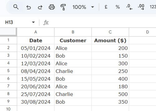
Goal: Extract the largest (latest) date per customer.
1. Find the Largest Date in Each Group Using QUERY
The QUERY function is the easiest way to get the latest date per group in one step.
Formula:
=QUERY(A1:B, "SELECT MAX(A), B WHERE A IS NOT NULL GROUP BY B", 1)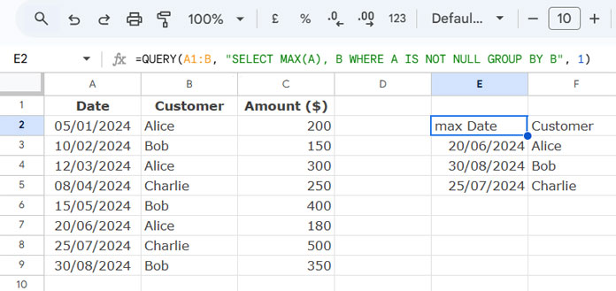
Steps to Use:
- Select a blank cell and enter the formula.
- Modify column references:
- Replace A1:B with your actual data range.
- Replace A with the date column letter.
- Replace B with the group column letter.
- Press Enter—this will return the latest date per group.
Pros: Simple and doesn’t require additional columns.
Limitation: Only returns the date and group column (not other columns).
2. Find the Largest Date in Each Group Using MAXIFS
The MAXIFS function is another efficient method. It works by filtering the maximum date for each unique group.
Step 1: Get Unique Groups
Enter this formula in cell E2 to extract unique customer names:
=UNIQUE(B2:B)Step 2: Find the Latest Date per Group
Enter this MAXIFS array formula in F2:
=MAP(E2:E, LAMBDA(val, IF(val="",,MAXIFS(A2:A, B2:B, val))))Explanation:
- E2:E -> Contains unique customer names.
- A2:A -> The date column.
- B2:B -> The customer column (group).
Pros: Works dynamically with multiple groups.
Limitation:
- Requires an additional UNIQUE column for groups.
- Uses LAMBDA, which may slow down performance in large datasets.
3. Find the Largest Date in Each Group Using SORTN
The SORTN function sorts and extracts the most recent entry per group.
Formula:
=SORTN(SORT(A2:B, 2, TRUE, 1, FALSE), 9^9, 2, 2, TRUE)How to Modify the Formula:
SORT(A2:B, 2, TRUE, 1, FALSE)- Replace
A2:Bwith the full data range. - Replace
2with the column number of the group column. - Replace
1with the column number of the date column.
- Replace
SORTN(..., 9^9, 2, 2, TRUE)- Replace the last
2with the column number of the group column.
- Replace the last
Pros: Can return all columns, unlike QUERY.
Limitation: Requires sorting support first.
Comparison: Best Formula to Use?
| Formula | Pros | Cons |
| QUERY | Simple, no extra columns | Returns only date & group column |
| MAXIFS | Works dynamically, easy to read | Requires UNIQUE column and LAMBDA support |
| SORTN | Can return all columns | Needs sorting first |
Best Choice?
- If you need a quick one-step formula -> Use QUERY
- If you want the dates and categories separately -> Use MAXIFS (it uses two standalone formulas).
- If you need all columns returned -> Use SORTN
Final Thoughts
To find the largest (latest) date in each group in Google Sheets, you can use QUERY, MAXIFS, or SORTN based on your needs. The QUERY method is the easiest, but MAXIFS and SORTN offer more flexibility.
Which method works best for your dataset? Let me know in the comments!