


")


")

")
")
 in Excel & Google Sheets")


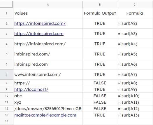
The ISURL function in Google Sheets is categorized under Web functions and is used to check if a value is a valid URL.
The ISURL formula returns TRUE or FALSE based on whether the provided input is a valid URL. If the formula returns TRUE, it recognizes the input as a valid URL.
In Google Sheets, URLs are typically displayed with blue, underlined text, but even if they aren’t visually linked, the ISURL function can still verify their validity.
Syntax
ISURL(value)- value: The value (supposed URL) to be verified.
ISURL Function: Example and Explanation
The ISURL function doesn’t require a URL to include “http” or “https” protocols, or the “www” subdomain, to return TRUE. A URL without these elements can still be considered valid.
Refer to the screenshot below for examples.
According to Google’s documentation, ISURL supports the following protocols:
- ftp
- http
- https
- gopher
- mailto
- news
- telnet
- aim
Additionally, note that the localhost domain (as shown in cell A9, with output in cell B9) is considered a valid URL in Google Sheets.
This means a top-level domain (TLD) like .com, .org, or .net is not necessary for a URL to be validated.
Using ISURL in Conditional Formatting
To highlight valid URLs in Google Sheets, you can use the ISURL function as a custom formula in Conditional Formatting.
Example:
Let’s say you want to highlight valid URLs in column A (range A2:A21). You can use this custom formula:
=ISURL(A2)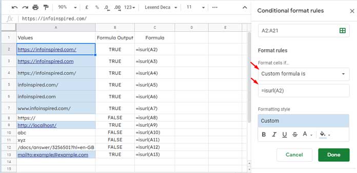
To apply this formula, first select the range you want to highlight and go to Format > Conditional formatting. Under the conditional formatting options (Format rules), select Custom formula is and enter the formula provided. Choose a formatting style and click Done.
Validating URLs with Data Validation
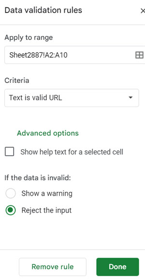
You can use Google Sheets’ built-in Data Validation rule to restrict data entry to valid URLs only.
Steps:
- Select the range where you want to allow valid URLs.
- Go to Data > Data validation.
- Click the +Add rule button.
- Under the Criteria dropdown, select Text is a valid URL.
- Click Done.
You can now enter only valid URLs in the selected range. For example, the settings below validate URL entries in the range A2:A10 in ‘Sheet2887’.
Checking URLs in Multiple Rows
To check URLs across multiple rows or columns, use the ArrayFormula function with ISURL.
Example:
To check URLs in the range A2:A13, use the following formula in B2, assuming that B2:B13 is blank.
=ArrayFormula(ISURL(A2:A13))Hyperlinking Valid URLs
You can create hyperlinks for valid URLs using a combination of the IF, ISURL, HYPERLINK, and ArrayFormula functions. Here’s an example formula that hyperlinks valid URLs in the range A2:A13:
=ArrayFormula(IF(ISURL(A2:A13), HYPERLINK(A2:A13), ""))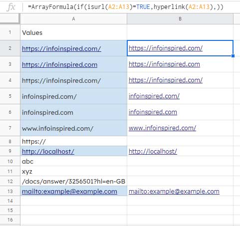
Related Reading
- Extract URLs from Hyperlinks in Google Sheets (No Scripting)
- UNIQUE Duplicate Hyperlinks in Google Sheets – Same Labels Different URLs
- How to Use ENCODEURL in Google Sheets to Create Clean URLs
- Extract Usernames from Email Addresses in Google Sheets
- How to Create a Hyperlink to an Email Address in Google Sheets
- ISEMAIL Function: Verify Email Addresses in Google Sheets