")
")


")


")

")
")
 in Excel & Google Sheets")


We can use the INDEX with MATCH or INDEX with XMATCH functions to return a 2D array result in Google Sheets. How is this possible?
Usually, the INDEX function returns the content of a cell based on the given row and column offsets. It can also return an entire single row or column.
For example:
=INDEX(A1:B, 5, 2)→ returns the value from the 5th row of the second column in the rangeA1:B.=INDEX(A1:B, 5, 0)→ returns the entire 5th row.=INDEX(A1:B, 0, 2)→ returns the entire 2nd column.
But how can we use INDEX to return a full 2D array in Google Sheets?
In spreadsheets, we specify ranges using a colon (:) between two references, e.g., B2:D10. Similarly, if we place a colon between two INDEX results, Google Sheets interprets that as a range and returns a matrix (2D array).
This trick opens up many possibilities in real-world scenarios.
Examples of INDEX with MATCH for 2D Arrays in Google Sheets
1. Copy a Table Up to a Matching Column
There are several ways to do this in Google Sheets. The simplest modern approach is with CHOOSECOLS + MATCH or XMATCH. But first, here’s how to do it with INDEX MATCH.
=INDEX(B2:B8):INDEX(B2:F8, 0, MATCH("Mar", B2:F2, 0))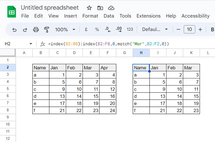
How it works:
- The left part (
INDEX(B2:B8)) returns the first column. - The right part (
INDEX(B2:F8, 0, MATCH("Mar", B2:F2, 0))) returns the column that matches"Mar". - Together, they form a range — just like writing
B2:E8— and return the full matrix.
Equivalent form:
=INDEX(B2:B8, 0, 0):INDEX(B2:F8, 0, 4)✅ Alternative using CHOOSECOLS + MATCH:
=CHOOSECOLS(B2:F8, SEQUENCE(MATCH("Mar", B2:F2, 0)))2. Extract Rows Based on a Value in Google Sheets
Suppose we want to find "b" in the first column, and also return that row plus the next two rows.
=INDEX(B2:B8, MATCH("b", B2:B8, 0)):INDEX(B2:F8, MATCH("b", B2:B8, 0)+2, 5)- The first INDEX returns the starting cell of the range (the cell containing “b”).
- The second INDEX offsets by 2 rows down and covers 5 columns.
- Combined, the result is the range
B4:F6.
This is another neat example of using INDEX MATCH to return a 2D array result in Google Sheets.
Examples of INDEX with XMATCH for 2D Arrays in Google Sheets
Like MATCH, we can also use XMATCH with INDEX. XMATCH is more flexible, especially when you need:
- To search from the last occurrence upward.
- To use wildcards for partial matches.
1. Extract Rows Between First and Last Occurrence
Suppose we have unstructured data and want to extract everything between "Orange" and "Orange Total".
=INDEX(B:B, XMATCH("Orange", B:B, 0)):INDEX(B:D, XMATCH("Orange*", B:B, 2, -1), 3)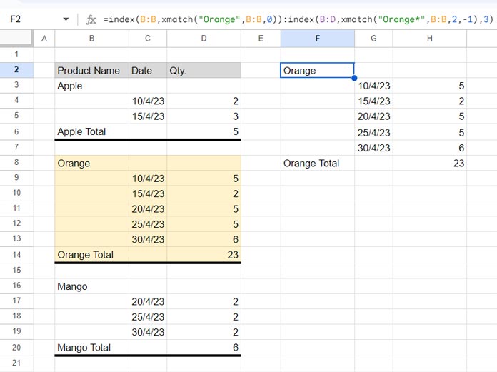
Explanation:
- The first
XMATCH("Orange", B:B, 0)finds the first"Orange"from top to bottom. - The second
XMATCH("Orange*", B:B, 2, -1)finds the last partial match (anything starting with"Orange") by searching bottom to top. - Two INDEX formulas joined with
:return the full matrix between these two points.
✅ This method works even when data is unstructured and other formulas like FILTER or QUERY struggle.
Why Use INDEX with MATCH or XMATCH for 2D Arrays in Google Sheets?
Using INDEX MATCH/XMATCH for 2D array results in Google Sheets is especially powerful when:
- You want matrix outputs, not just single-cell lookups.
- Your data is unstructured or doesn’t fit neatly into FILTER/QUERY use cases.
- You need flexibility with wildcards, last-to-first lookups, or dynamic ranges.