


Array result means result in a range instead of in a single cell. In some cases, we can use the IFS function to return an array result in Google Sheets.
To evaluate multiple conditions (criteria), we can use IF, SWITCH, or IFS. IF, which is so popular among these functions, requires nesting (multiple IF functions combined) that makes it look complicated.
Must Read: How to Use IFS Logical Function in Google Sheets [Also Nested IF].
The latter two functions are easy to use but lack at some point when compared to IF. That’s in the ability to return an array result.
In this post, I am going to elaborate on how to use the IFS function to return an array/range result in Docs Sheets. What else? I will also explain the alternative solution to return an array result when IFS fails.
Of course, we should only think about the IFS alternative, if we feel the IF nesting is tough to code and read later.
IFS Function to Return Result in a Range in Google Sheets
I have two examples.
- To show how to use IFS logical function to return an array result in Google Sheets.
- The other example is to show you where the IFS fails to return a range result.
In the second option, to replace IFS, we can use nested IF or Vlookup. Vlookup? Yes! It’s also an option.
IFS Function That Correctly Returns an Array Result in Google Sheets
Straightaway to one formula example.
I have the names of the days of week entered in a range as below.
| Sunday |
| Monday |
| Tuesday |
| Wednesday |
| Thursday |
| Friday |
| Saturday |
Assume, these are entered in the range A1:A7 in Google Sheets. What I want is to return 1 for Sunday, 2 for Monday, 3 for Tuesday and so on.
Here is the IFS array formula.
=ArrayFormula(ifs(A1:A7="Sunday",1,A1:A7="Monday",2,A1:A7="Tuesday",3,A1:A7="Wednesday",4,A1:A7="Thursday",5,A1:A7="Friday",6,A1:A7="Saturday",7))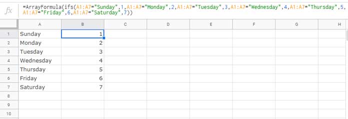
When we use IFS function to return an array result as above, we may face one issue. What’s that?
Assume if one of the logical expression is FALSE. As an example delete the value in cell A3. We can see that the formula returns N/A error in cell B3. It’s because, unlike IF, IFS doesn’t contain the value_if_false argument.
There are two methods to overcome this drawback in IFS which I have detailed in one of my earlier guide – How to Return Value When The Logical Expression is FALSE in IFS.
Here in our above example, we can execute the value_if_false argument as below.
=ArrayFormula(ifs(A1:A7="Sunday",1,A1:A7="Monday",2,A1:A7="Tuesday",3,A1:A7="Wednesday",4,A1:A7="Thursday",5,A1:A7="Friday",6,A1:A7="Saturday",7,1=1,"?"))Simply replace the question mark (see the end part of the formula) with the value you want.
If the value you want to return is a string, keep the double-quotes, else if it’s a number remove the double-quotes.
Similar to number, if the FALSE part in IFS is a date or time, use the functions DATE or TIME respectively.
Example:
=ArrayFormula(ifs(A1:A7="Sunday",1,A1:A7="Monday",2,A1:A7="Tuesday",3,A1:A7="Wednesday",4,A1:A7="Thursday",5,A1:A7="Friday",6,A1:A7="Saturday",7,1=1,date(2019,8,28)))If it’s a time it should be entered in the format – TIME(hour, minute, second).
Google Sheets IFS Formula Fails to Return a Range
Let me show you one instance where the IFS fails to return a range result. Assume you want to evaluate one value and if evaluates to TRUE, return two or more values.
Example:
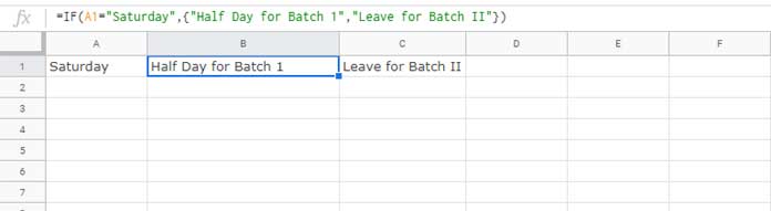
The value to evaluate in cell A1 is a string which is “Saturday”.
=IF(A1="Saturday",{"Half Day for Batch 1","Leave for Batch II"})This IF formula in cell B1 will return an array result in cell B1 and C1.
But the following IFS formula will only return the value “Half Day for Batch 1”.
=IFS(A1="Saturday",{"Half Day for Batch 1","Leave for Batch II"})No matter whether we use ArrayFormula function with it as below.
=ArrayFormula(IFS(A1="Saturday",{"Half Day for Batch 1","Leave for Batch II"}))The IFS formula miserably fails to return an array result here. I don’t want to use IF here. Is there any alternative solution?
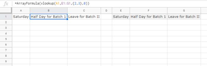
Vlookup can replace IFS in the above example.
Vlookup as an Alternative to IFS Range Output
Formula:
=ArrayFormula(vlookup(A1,{A1,"Half Day for Batch 1","Leave for Batch II"},{2,3},0))In real-life use, to simplify the above Vlookup, we can call the range from outside (as cell reference).
Related Reading: How to Correctly Use AND, OR Functions with IFS in Google Sheets.