The LET function in Google Sheets is all about assigning names to expressions.

We can call the assigned name multiple times in a formula instead of the expression itself.

There are two main benefits of using such names instead of expressions.

1. It improves the readability of the formula, especially for a third person or for yourself on a future date.
2. It offers better performance.

I know I must explain these two points further.

Readability:

Assume we have a formula that returns the sum of a range of cells. E.g., total sales in a month.

=sum(C:C)

We can use the IF function to test whether the total sales meet our target. It would be like this.

=if(sum(C:C)<100,"d",if(sum(C:C)<200,"c",if(sum(C:C)<300,"b","a")))

We can use the LET Google Sheets function to name sum(C:C) with the variable x and thus shorten the formula.

So you only require to use the sum(C:C) formula one time and can replace all other occurrences with the name variable x.

Performance Improvement:

If you write the same expression multiple times in a formula, in the above example it’s sum(C:C), Google Sheets will calculate that result multiple times.

That will affect the performance, especially when the formula is complex.

Syntax of the LET Function in Google Sheets

Syntax: LET(name1, value_expression1, [name2, …], [value_expression2, …], formula_expression)

Arguments:

name1, [name2, …]: The names to assign to the value_expression1, [value_expression2, …].

Please note that the usage of these name arguments in the LET function is case-insensitive.

value_expression1, [value_expression2, …]: The assigned values to name1, [name2, …].

formula_expression: A calculation that uses name1, [name2, …] within the LET function.

Note:

All the arguments in the square brackets are optional. If you specify name2, you must specify value_expression2 also. But not necessarily within the formula_expression.

Here are a few examples of the LET function in Google Sheets.

Basic Examples

Here are two examples that show how to use the LET function in Google Sheets. We will use a name and a value expression in the first example.

=let(a,5,a*2)

Result: 10

In this LET formula, a is the name1, 5 is the value_expression1, and a*2 is the formula_expression.

Below, you can see how to use two names and two value expressions.

=let(a,5,b,2,a*b)

Result: 10

Real-life Use of the LET Function in Google Sheets

The above two formulas are to explain the usage of the LET function in Google Sheets.

We won’t be using the function in that way in real life.

Here is one real-life use example of the LET function in Google Sheets.

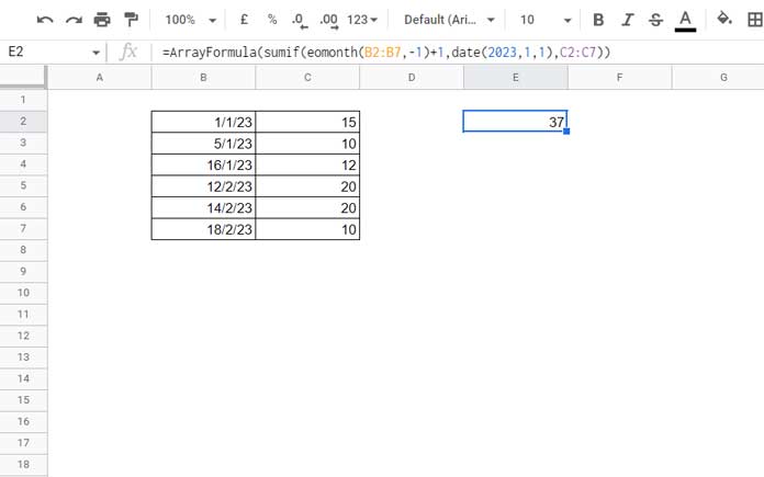
When we want to sum a numeric column based on a criterion, one of the functions that we can depend on is the SUMIF function.

To sum the sales amount (C2:C7) in January 2023 (B2:B7), we can use the following SUMIF formula in Google Sheets.

=ArrayFormula(sumif(eomonth(B2:B7,-1)+1,date(2023,1,1),C2:C7))

Now I would like to test this result and return “poor” if the result is <10, “good” if it is >=10, and <40, and “exceptional” if it’s >=40.

I may suggest using the following IF logical test for that.

=if(ArrayFormula(sumif(eomonth(B2:B7,-1)+1,date(2023,1,1),C2:C7))<10,"poor",if(ArrayFormula(sumif(eomonth(B2:B7,-1)+1,date(2023,1,1),C2:C7))<40,"good","exceptional"))

There are two problems with this formula, which we can sort out using the LET function.

What are those problems?

1. The formula is not reader-friendly.
2.  Google Sheets evaluates the monthly sum (SUMIF) twice.

Here is the LET alternative.

=let(x,ArrayFormula(sumif(eomonth(B2:B7,-1)+1,date(2023,1,1),C2:C7)),if(x<10,"poor",if(x<40,"good","exceptional")))

name_1: x

valule_expression1: ArrayFormula(sumif(eomonth(B2:B7,-1)+1,date(2023,1,1),C2:C7))

formula_expression: if(x<10,"poor",if(x<40,"good","exceptional"))

LET and LAMBDA

Though we can replace the above LET formula with a LAMBDA, I don’t suggest replacing the former with the latter because the purpose of the LAMBDA is different.

What are those purposes?

1. The LAMBDA has helper functions, such as BYROW, BYCOL, SCAN, REDUCE, MAP, and MAKEARRAY. These LHFs are native Google Sheets functions that use LAMBDA to perform advanced array operations.
2. When you want to test a custom-named function within Sheet, use a LAMBDA.

If we replace the above LET with a LAMBDA, it would be as follows.

=lambda(x,if(x<10,"poor",if(x<40,"good","exceptional")))(ArrayFormula(sumif(eomonth(B2:B7,-1)+1,date(2023,1,1),C2:C7)))

That’s all about the LET function in Google Sheets. Thanks for the stay. Enjoy!