I’m going to share with you a rare and tricky way to use AND and OR logic with the Google Sheets FILTER function. We won’t use the AND and OR functions directly, but instead, we’ll leverage the plus (+) and asterisk (*) operators.
Additionally, I will compare the AND, OR, and FILTER combination with the AND, OR, and IF combination.
We already have detailed tutorials on these functions.
Different Scenarios for Combining AND, OR, and FILTER in Google Sheets
There are three scenarios for using the FILTER formula with logical operators: filtering based on OR criteria, filtering based on AND criteria, and using a combination of AND and OR within the FILTER formula.
Let me explain the type of data we are going to filter using this combination of functions.
Sample Data:
Student names in A2:A4 and their marks in Maths, Physics, and Chemistry in B2:D4.
| Name | Maths | Physics | Chemistry |
| Jo Griffin | 51 | 16 | 24 |
| Emilio Mccormick | 50 | 48 | 80 |
| Lena Pena | 92 | 93 | 79 |
We will set up three different passing conditions for the exam based on student scores:
- Passing any subject: Students need to score more than 49 marks in at least one subject. (This uses OR logic)
- Passing all subjects: Students must score more than 49 marks in all three subjects. (This uses AND logic)
- Passing two subjects: Students need to score more than 49 marks in any two subjects. (This combines AND and OR logic)
We’ll explore how to check these scenarios using both the FILTER, AND, OR combination and the IF, AND, OR combination in Google Sheets.
Examples
We have six formulas in total: three using IF, AND, and OR logic, and three using the FILTER function with combinations of AND and OR logic.
OR with FILTER Function (Any One Subject >= 50, Passed)
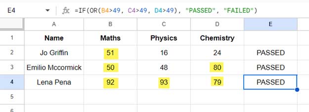
First, let’s see how to address this scenario using the IF and OR combination. Enter the following formula in cell E2 and drag the fill handle down:
=IF(OR(B2>49, C2>49, D2>49), "PASSED", "FAILED")It will return “PASSED” in E2, E3, and E4.

Here, the OR function tests whether the marks in B2, C2, or D2 are greater than 49. If it evaluates to TRUE, the IF function returns “PASSED”; otherwise, it returns “FAILED”.
OR and FILTER Combo:
=IFERROR(FILTER(A2:A4, (B2:B4>=50)+(C2:C4>=50)+(D2:D4>=50)))This will output the names of passed students.
| Jo Griffin |
| Emilio Mccormick |
| Lena Pena |
This formula adheres to the syntax FILTER(range, condition1, [condition2, …]).
The range to filter is A2:A4, which contains the names of the students. The condition is (B2:B4>=50)+(C2:C4>=50)+(D2:D4>=50).
This will return 1, 2, and 3 for the rows corresponding to the first, second, and third students, respectively.
The FILTER function filters the names wherever the condition is greater than 0. So, it will return all the names, meaning all the students have passed.
AND with FILTER Function (All Subjects >= 50, Passed)
In this scenario, we want to switch the logic in the IF statement from OR to AND. We can achieve this by using the asterisk (*) operator instead of the plus (+) operator in the FILTER formula’s condition.
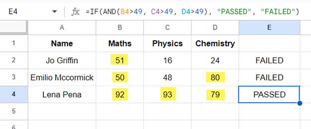
Here is the IF and AND combination for cell E2:
=IF(AND(B2>49, C2>49, D2>49), "PASSED", "FAILED")Drag the E2 fill handle to E4.

This formula returns “PASSED” if all the conditions are met; otherwise, it returns “FAILED.”
And here is the use of the AND logical test in FILTER:
=IFERROR(FILTER(A2:A4, (B2:B4>=50)*(C2:C4>=50)*(D2:D4>=50)))This formula filters the names in the rows where all the conditions return true, meaning equal to 1.
Output:
| Lena Pena |
However, when using AND with FILTER, it’s not necessary to rely on the * operator. You can specify the conditions separately as shown below:
=IFERROR(FILTER(A2:A4, B2:B4>=50, C2:C4>=50, D2:D4>=50))AND and OR with FILTER Function (At Least Two Subjects >= 50, Passed)
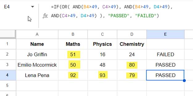
This formula uses a combination of IF, AND, OR logic to determine if a student passes. It checks if any two subjects have scores greater than 49. The formula will return ‘PASSED’ if any two subjects have scores above 49, and ‘FAILED’ otherwise. Enter it in cell E2 and drag the E2 fill handle to E4.
=IF(OR( AND(B2>49, C2>49), AND(B2>49, D2>49), AND(C2>49, D2>49) ), "PASSED", "FAILED")
And here’s the FILTER formula with AND and OR logic:
=IFERROR(FILTER(A2:A4, ((B2:B4>=50)*(C2:C4>=50)) + ((B2:B4>=50)*(D2:D4>=50)) + ((C2:C4>=50)*(D2:D4>=50)) ))This formula uses the FILTER function to return the names (from A2:A4) of students who scored greater than or equal to 50 in at least two subjects (B2:B4, C2:C4, D2:D4)
| Emilio Mccormick |
| Lena Pena |
The formula uses multiplication (*) to combine AND logic within each condition. It then adds (+) these conditions using OR logic. This means it checks if a student has a score of 50 or higher in Maths and Physics, OR Maths and Chemistry, OR Physics and Chemistry.
Be sure to carefully check all the formulas and experiment with your own dataset to learn this trick.


Is there any way to add both types of functions for the filer?
To use criterion 1 and criterion 2 or criterion 3.
Below is what I have for two criteria that need to be inputted. But I want to make the third criterion optional or leave it blank.
=FILTER(pricebooks_data,Pricebook_name=B3,Currency=B4)The above works.
=FILTER(pricebooks_data,Pricebook_name=B3,Currency=B4 OR(Product_family=B5))It doesn’t work.
Hi, Caroline,
Here is one way to solve this.
=FILTER(pricebooks_data,Pricebook_name=B3,Currency=B4,if(B5="",row(Product_family),Product_family=B5))
Related: Select All or a Specific Category in Multiple Columns in Filter in Google Sheets.
Many thanks to you! I had similar questions / needs to Heather and Nicholas, and this was the only tutorial I found that addressed it. Much appreciated!
Hi, Milo,
Thanks for your feedback.
THANK YOU!!
I’ve been trying to find this Filter AND/OR solution for weeks in my spare time. I knew there had to be a way.
Thank you for the excellent tutorial!
I’m trying to create a filter formula with multiple OR conditions, that is more open-ended. This formula is working for me.
=filter(A3:C, (A3:A = E3)+(A3:A = E4)+(A3:A = E5))However, column E is meant to be dynamic and updating.
I have tried Query to do the same, but have run into similar issues with an open range.
The fixed range equation looks like this –
=query({Example!A3:C}, "Select * where Col1 matches "&ArrayFormula("'"&textjoin(".*|",true,".*"&E3:E5)&".*'")& "order by Col1 asc")Thank you for any help you can offer and for your excellent tutorials!
Much of what I know about Google Sheets, I have learned from your site!
Hi, Anne-Marie,
You were almost close to the solution with your Query()
Replace
E3:E5withfilter(E3:E,len(E3:E))If you want Filter(), go with this one.
=filter(A3:C, regexmatch(A3:A,"(?i)^"&textjoin("$|^",true,E3:E)&"$"))Thank you so much for the Advanced Filter AND OR combination. I tried with “,” together with “+”, but it did not work. The key was to replace the “,” with a “*” to get it to work! Thx!
Hi,
Can we use importrange with a combination of Filter and OR?
Hi, Hima,
Yes! We can do that. But not advisable because it might slow down the performance of the file (sheet).
The reason we need to use multiple importrange formulas. One importrange for ‘range’ another for ‘condition1’ and so on.
FILTER(range, condition1, [condition2, …])So better to use Query as multiple OR is easy to use in Query.