The basic purpose of the ADDRESS function in Google Sheets is to return a cell reference, given a row and column input. What makes it even more powerful is that we can use functions like MATCH, XMATCH, ROW, and COLUMN to replace the row and column arguments.

The MATCH and XMATCH functions are two lookup functions. You can use them with ADDRESS to return the cell reference of a lookup value.

Let’s first see how to use the ADDRESS function in Google Sheets, because it can return relative and absolute references, as well as sheet names.

ADDRESS Function in Google Sheets: Syntax and Arguments

Syntax of the ADDRESS function in Google Sheets:

ADDRESS(row, column, [absolute_relative_mode], [use_a1_notation], [sheet])

Cell reference examples (in A1 style notation):

$A$1, A$1, $A1, and A1

The ADDRESS function can return all four types of cell references, which play a key role in Conditional Formatting.

Argument explanations:

Out of the five arguments, the first two are required and the rest of the three are optional. The tick mark shows what the function uses if the optional arguments are omitted.

• row: The row number part of the cell reference. For example, 100 in Z100.
• column: The column number part of the cell reference. A is column number 1. For example, 26 in Z100.
• absolute_relative_mode: (Optional) An indicator of whether the returned cell reference is absolute or relative:
  • 1 is row and column absolute (e.g., $A$1). ✅
  • 2 is row absolute and column relative (e.g., A$1).
  • 3 is row relative and column absolute (e.g., $A1).
  • 4 is row and column relative (e.g., A1).
• use_a1_notation: A boolean indicating whether to use A1 style notation (TRUE ✅) or R1C1 style notation (FALSE).
• sheet: (Optional) To include a sheet name (Absent ✅ by default).

ADDRESS Function Formula Examples (with Explanations)

The following formula would return $Z$10 because the row argument is 10 and the column argument is 26:

=ADDRESS(10,26)

In this result, both row and column references are absolute. To make them relative, we can use the third argument, which is absolute_relative_mode:

=ADDRESS(10,26,1) // returns $Z$10
=ADDRESS(10,26,2) // returns Z$10
=ADDRESS(10,26,3) // returns $Z10
=ADDRESS(10,26,4) // returns Z10

How do we specify the sheet name to point to in an ADDRESS formula?

Let’s use the fifth argument, sheet. Here is an example:

=ADDRESS(10,26,4,,"form_response") // returns 'form_response!'!Z10

As you can see, we haven’t used the fourth argument, which is use_a1_notation. That’s why we left a comma immediately after the third argument in the formula.

The following ADDRESS formula returns the cell address in R1C1 reference style:

ADDRESS(10,1,1,FALSE) // returns R10C1

You can use the INDIRECT function with the ADDRESS function to return the cell value of the cell reference returned by the latter function.

In all the formulas, except the last one which returns R1C1 style cell reference, you just wrap the formula with INDIRECT.

Example:

=INDIRECT(ADDRESS(10,1))

This formula will return the cell value of A10.

When using R1C1 notation, use the formula as follows:

=INDIRECT(ADDRESS(10,1,1,FALSE),FALSE)

How to Use Dynamic Row and Column Arguments in the ADDRESS Function

To find the cell address of the first or last occurrence of a value in a range, you can use the XMATCH function within the ADDRESS function. Let’s see how to use it as a dynamic row or column in the ADDRESS function in Google Sheets.

Using the XMATCH Function to Create Dynamic Row Arguments

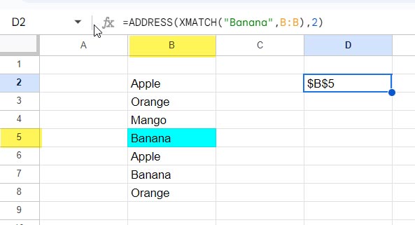
For example, assume that column B contains fruit names. The following XMATCH formula will return the row number of the first occurrence of “Banana” in that column:

XMATCH("Banana",B:B)

We can then use this XMATCH formula to replace the row argument in the ADDRESS function:

=ADDRESS(XMATCH("Banana",B:B),2)

Where:

• row is XMATCH("Banana", B:B)
• column is 2

This formula will return $B$5, as per the sample data in the screenshot below.

To get the cell address of the last matching value, use the following ADDRESS and XMATCH combo.

=ADDRESS(XMATCH("Banana",B:B,0,-1),2) // returns $B$7

Using the XMATCH Function to Create Dynamic Column Arguments

If your data is arranged in a row, replace the column argument in the ADDRESS function with the XMATCH function.

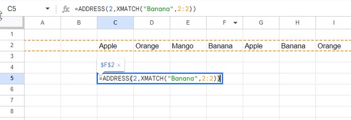
The following formula will return the cell address of the first occurrence of the fruit “Banana” in row # 2:

=ADDRESS(2,XMATCH("Banana",2:2)) // returns $F$2

To get the cell address of the last occurrence of the value “Banana” in that row, use the following formula instead:

=ADDRESS(2,XMATCH("Banana",2:2,0,-1)) // returns $H$2

Using the XMATCH Function to Create Dynamic Row and Column Arguments in the ADDRESS Function

Sometimes, we may want to use dynamic row and column arguments in the ADDRESS function to get the cell address of an intersection of two matching values. To do this, we can use two XMATCH formulas: one for replacing the row argument and the other for replacing the column argument.

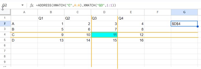
The following formula will match the value “C” in column A and “Q3” in row #1 and return the cell address of the intersection value:

=ADDRESS(XMATCH("C",A:A),XMATCH("Q3",1:1))

The beauty of this formula is that to get the value itself, you can just wrap it with INDIRECT.

=INDIRECT(ADDRESS(XMATCH("C",A:A),XMATCH("Q3",1:1))) // returns 11

Note: You can replace XMATCH with MATCH in the ADDRESS function, but this will not support matching the last value.

How to Use ADDRESS Function Array Formulas in Google Sheets

We have seen a few advanced uses of the ADDRESS function above. Here are a few more examples:

We can use the ADDRESS function to match a value in multiple cells in a row, column, or range and return the cell addresses of all of the matches.

For example, the following array formula will return the cell addresses of all cells in column A that contain the value “Apple”:

=ARRAYFORMULA(
   TOCOL(
      IF(
         A:A="Apple",
         ADDRESS(ROW(A1:A),COLUMN(A1:A)),
      ),1
   )
)

The ADDRESS function returns the cell address of a cell based on its row and column numbers. The IF function checks each cell in the range A:A to see if it contains the value “Apple”. If it does, the IF function returns the cell address of that cell. Otherwise, the IF function returns an empty string (“”).

The TOCOL function is just for removing the blank cells in the result.

When you use this formula in a row, replace the function TOCOL with the function TOROW. The following formula is for row #1:

=ARRAYFORMULA(
   TOROW(
      IF(
         1:1="Apple",
         ADDRESS(ROW(1:1),COLUMN(1:1)),
      ),1
   )
)

To use the ADDRESS function in a range (2D array) to return multiple cell addresses, you can use the following array formula:

=ARRAYFORMULA(IF(B2:E5="",,ADDRESS(ROW(B2:E5),COLUMN(B2:E5))))

This formula will return the cell addresses of all non-empty cells in the range B2:E5.