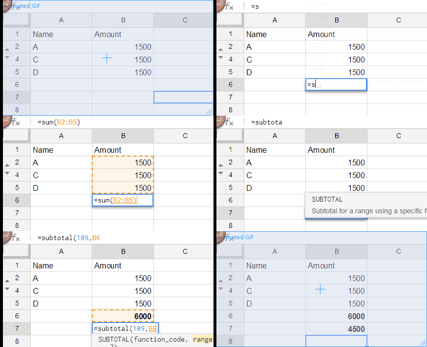
You can omit hidden or filtered-out values in the sum in Google Sheets, but not with the normal SUM function. For this purpose, you should use the SUBTOTAL function with function code 9 (omits/excludes filtered-out rows) or 109 (omits/excludes filtered-out and hidden rows). So, this post is actually about how to use the SUBTOTAL function in Google Sheets to sum visible rows.
Google Docs Spreadsheet has several Excel-like functions to meet users’ data entry needs. The SUBTOTAL is one such function. Functions like QUERY, REGEXMATCH, and IMPORTRANGE make Google Sheets a perfect spreadsheet solution that others envy.
As a side note, you can refer to my Google Sheets Functions guide to learn all the popular Google Sheets functions with examples.
Formula to Omit Hidden or Filtered Out Values in Sum
We will start with a basic example that uses the source data and formula within the same sheet. Next, we will see how to use the source data in one sheet and the formula in another sheet, but within the same workbook. Finally, we will see how to omit hidden or filtered-out values when the source data is in one file and the formula is in another file.
Source Data and SUBTOTAL Formula in the Same Sheet
I have the values to sum in B2:B5. Let’s see how to exclude values in hidden rows or filtered-out rows in a total in cell B7.
Notes:
- Filtered out means filtering records using Data > Create a filter or Data > Add a slicer.
- Hidden rows means hiding records using the right-click menu on a row and clicking Hide, or by applying grouping to selected rows using the View > Group feature.
As clearly stated above, to make a total or sum that excludes hidden or filtered-out rows, you should use the SUBTOTAL() function instead of the SUM() function.
You must use the sum function code, i.e., 9 or 109 because the SUBTOTAL function is capable of eleven types of aggregation.
In the following example, I’ve hidden row #3 by right-clicking on it and choosing Hide from the shortcut menu.
=SUBTOTAL(109,B2:B5)
When the SUM function adds the value in the hidden row to the total, the SUBTOTAL function omits it.
The same will happen if you apply the SUBTOTAL function to a filtered table.
If you only want to omit the filtered-out rows, replace the SUM function code 109 with 9 in the formula. It will include hidden rows.
Source Data and SUBTOTAL Formula in Two Different Sheets in the Same File
If the above range to sum is in Sheet1, use the following formula:
=SUBTOTAL(9,Sheet1!B2:B5)You can use this formula in Sheet1 or any other sheet in the same file.
How to Omit Hidden or Filtered-Out Values in Sum in IMPORTRANGE Data
We use the IMPORTRANGE function to import data from one Google Sheets file to another. You can import data easily using this function.
To do this, you need to specify only two arguments: the URL of the Google Sheets file from which you want to import the data and the sheet name with range.
For example, the following formula in cell A1 will import the range B2:B5 in Sheet1:
=IMPORTRANGE("https://docs.google.com/spreadsheets/d/1as2K3NyJ58WipNSm56rtE__-DD3F6_x_RAp2ElpHNJw/edit#gid=1892488864","Sheet1!B2:B5")Note: This formula will not work for you because I used a dummy URL for the demonstration. You need to replace the URL with the URL of the sheet containing the data to import.
You can wrap this formula with SUM to get the total of the imported values:
=SUM(IMPORTRANGE("https://docs.google.com/spreadsheets/d/1as2K3NyJ58WipNSm56rtE__-DD3F6_x_RAp2ElpHNJw/edit#gid=1892488864","Sheet1!B2:B5"))How do we omit hidden or filtered-out values in the sum of this imported data? Wrapping it with SUBTOTAL doesn’t work because the SUBTOTAL argument must be a range, and we are providing it an expression instead.
Workaround:
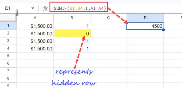
In the source sheet, insert the following MAP formula in cell C2 (C2:C5 must be blank beforehand):
=MAP(B2:B5, LAMBDA(row, SUBTOTAL(103,row)))Import B2:C5 instead of B2:B5.
=IMPORTRANGE("https://docs.google.com/spreadsheets/d/1as2K3NyJ58WipNSm56rtE__-DD3F6_x_RAp2ElpHNJw/edit#gid=1892488864","Sheet1!B2:C5")Use the following SUMIF formula instead of SUM.
=SUMIF(B1:B4,1,A1:A4)
This way, we can omit hidden or filtered-out values in the sum of imported data in Google Sheets.
Related:


It’s not working for me. I need it to sum only cells that return a value of 1 which is Attended.
Hi, Lazaro,
I think you are asking about conditional subtotal. I have included the related tutorial link inside the post. If you fail to find it you can Share an example Sheet with me. In that Sheet replicate your problem and the result you want.
Best,
Awesome thanks so much!!!
Thanks for the tip!
I didn’t get why 109 though?
Hi, It’s function number for sum to be used in subtotal.
Hi,
Here is all about Function Numbers!
https://infoinspired.com/google-docs/what-is-function-numbers-in-google-sheets/
Cheers!
Excellent tip, very useful!