


")


")

")
")
 in Excel & Google Sheets")


You can highlight VLOOKUP results in Google Sheets mainly in two ways, which we will explore below:
- Highlight the lookup result within the lookup table.
- Highlight values in a list if they are present in the lookup table and meet a condition.
Option 1: Highlight VLOOKUP Results within the Lookup Table
In the following example, I want to look up the name “David” in cell A1 in the lookup table (B2:D7) and highlight the marks in the third column.
When I change the name in cell A1 to another name, the highlighting should be updated accordingly.
How do we highlight VLOOKUP results in Google Sheets as described above?
Since VLOOKUP doesn’t work directly with Conditional Formatting in this way, we need to find the cell address of the VLOOKUP result and use that to match each cell in the table for conditional formatting.
Step 1: Find the Row Number of the Lookup Value
We can use the MATCH function for this:
=MATCH($A$1, $B$2:$B$7, FALSE)+ROW($B$2)-1Syntax:
MATCH(search_key, range, [search_type])Where:
search_key: $A$1 (lookup value)range: $B$2:$B$7 (range to lookup)search_type: FALSE (exact match)
The lookup range starts from the second row. To convert the relative position of the search key in the range to the actual row number, we add ROW($B$2)-1. Adding 1 directly won’t adjust the range if you move your table in the future.
Step 2: Find the Column Number of the VLOOKUP Result
To get the column number for column D:
=COLUMN($D$2)Step 3: Find the VLOOKUP Result Cell Address
We can use the ADDRESS function to get the VLOOKUP result cell reference as a string by using the row and column numbers obtained above:
=ADDRESS(MATCH($A$1, $B$2:$B$7, FALSE)+ROW($B$2)-1, COLUMN($D$2))Next, we can use this cell reference to highlight the VLOOKUP result.
Step 4: Highlight VLOOKUP Results within the Lookup Table
Match each cell reference in the lookup table with the VLOOKUP result address (step 3 output) within Conditional Formatting. Here’s how:
- Get the Address of the First Cell in the Range:
=CELL("address", B2)– This is just for your reference. - Match it with the VLOOKUP Result Cell Address:
=CELL("address", B2)=ADDRESS(MATCH($A$1, $B$2:$B$7, FALSE)+ROW($B$2)-1, COLUMN($D$2))– This formula will be used in Conditional Formatting. - Apply Conditional Formatting:
- Select the lookup table range B2:D7.
- Click Format > Conditional formatting.
- Under Format rules, select Custom formula is.
- Copy and paste the above formula into the field.
- Choose a formatting style under Formatting style.
- Click Done.
This approach dynamically updates the formatting when you move the table by inserting rows or columns, as it uses dynamic references.
Option 2: Conditional Formatting for Lookup Values Present in Another Table
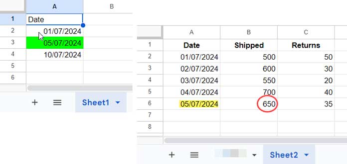
This scenario involves search keys in column A of Sheet1. We want to look up these values in a table in Sheet2 and highlight the values in column A (Sheet1) if they match a condition.
For example, consider the table in A1:C6 in Sheet2:
| Date | Shipped | Returns |
| 01/07/2024 | 500 | 50 |
| 02/07/2024 | 600 | 30 |
| 03/07/2024 | 550 | 20 |
| 04/07/2024 | 700 | 40 |
| 05/07/2024 | 650 | 35 |
In Sheet1, we have the following dates in A1:A, where A1 contains a field label:
| Date |
| 01/07/2024 |
| 05/07/2024 |
| 10/07/2024 |
We want to highlight this list if the shipped quantities for these dates in Sheet2 are greater than 600.
The following VLOOKUP formula will look up the search key in Sheet1!A2 in Sheet2!A1:C6 and return the shipped value on that particular date:
=VLOOKUP(A2, Sheet2!$A$1:$C$6, 2, FALSE)To test whether the value is greater than 600, use:
=VLOOKUP(A2, Sheet2!$A$1:$C$6, 2, FALSE)>600However, this won’t work directly in Conditional Formatting. When the custom rule contains a cell or range reference in a different table, you should indirectly refer to them as follows:
=VLOOKUP(A2, INDIRECT("Sheet2!A1:C6"), 2, FALSE)>600How to apply this rule:
- Select the range A2:A or up to the row from A2 in Sheet1.
- Click Format > Conditional formatting.
- Select Custom formula is under Format rules.
- Copy and paste the above formula in the field immediately below.
- Click Done.
This is another option to highlight VLOOKUP results in Google Sheets. Here, we are highlighting the search keys if the VLOOKUP result meets a certain criterion.
Additional Tip
You can use the FILTER function as an alternative to the VLOOKUP method described above. Replace the highlighting rule with the following FILTER formula:
=FILTER(INDIRECT("Sheet2!B2:B6"), INDIRECT("Sheet2!A2:A6")=A2)>600