This post has the potential to be a valuable time-saving tip for many beginners working with Google Docs Spreadsheets. Here, you’ll delve into a common spreadsheet task: filtering, but with a unique approach.
In Google Sheets, there are two functions, FILTER and QUERY, that can be employed to filter data. However, when it comes to filtering data to separate sheets within the same workbook, the FILTER function is the method of choice, as opposed to QUERY. This is because the latter does not retain hyperlinks.
Typically, the filter menu command is utilized to sift through large datasets, aiding in the focus on relevant information. By utilizing the FILTER function in Google Sheets, you can efficiently filter data, essentially transferring filtered data to different sheets.
Now, what exactly does it mean to filter data with links?
This concept has two implications:
- The filtered data will automatically update when changes are made to the source data.
- The filtered data will not lose any hyperlinks.
Filtering Data to Separate Sheets: Can It Be Done in Excel Too?
You can filter data to separate sheets or ranges in Microsoft Excel using the advanced filter option. However, there’s a distinction with the FILTER function in Google Sheets.
The FILTER function in Google Sheets copies the filtered data with links to other tabs or ranges. This means that changes in your master data will be reflected in your filtered data, and any hyperlinks will be retained.
Update: The FILTER function is now available in Excel as well (not in all versions), though the usage might be slightly different.
Tips for Transferring Filtered Data with Links to Different Sheets or Sheet Tabs
Here, we are going to use the FILTER function in Google Docs Spreadsheet. The syntax is as follows:
Syntax:
FILTER(range, condition1, [condition2, …])The entire process is straightforward if you follow the spreadsheet tutorial below. Just refer to the example to master the FILTER function and apply it later as needed.
Steps
Step 1:
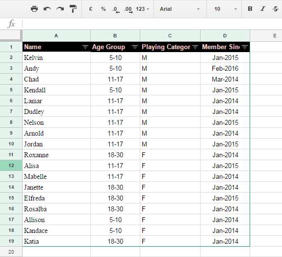
Enter the following data in a new Google Sheets spreadsheet or copy my sample sheet with the sample data and all the formulas by clicking the button immediately after the image.

You can observe from the above data that it is a list of the members of a club.
We are going to filter the members’ names based on their age group. There are three different age groups in this sample data [see column B, i.e., “Age Group”].
Step 2:
Create three new tabs or sheets and name them as follows: ‘Age Group 5-10,’ ‘Age Group 11-17,’ and ‘Age Group 18-30.’

Step 3:
Copy the column header to the first row of each of the newly created sheets.

Step 4:
This is the final step. Apply the function to the second cell of each new tab, i.e., cell A2.
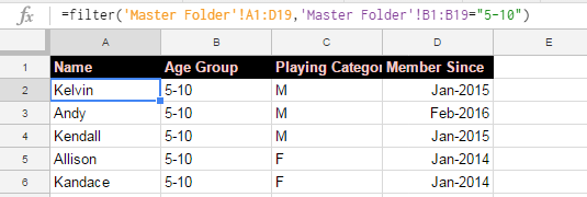
The formula for the first tab is:
=FILTER('Master Folder'!A1:D19,'Master Folder'!B1:B19="5-10")
Please don’t get confused with the formula. Check the syntax given above. We want to select the range and provide the filter criteria.
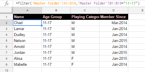
The formula for the second tab is:
=FILTER('Master Folder'!A1:D19, 'Master Folder'!B1:B19="11-17")
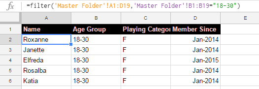
The formula for the third tab is:
=FILTER('Master Folder'!A1:D19, 'Master Folder'!B1:B19="18-30")
This will automatically generate the filtered data in the newly created sheets. That’s it!
Conclusion
Now you have a total of four sheets. The first one is the master dataset, and the other three contain the filtered data. Remember to change the cell reference in the formula in each sheet if you add more rows to your master data later. Alternatively, you can use open-ended ranges such as A1:D and B1:B instead of A1:D19 and B1:B19.
The sample data may have hyperlinks. If it does, the FILTER function will transfer them along with the filtered data. When you hover your mouse pointer over the text, you can see the clickable link.
Will the above filtered data in separate sheets refresh when we add or delete data in the source sheet?
Yes, it will. If you want to explore advanced filtering, please check my tutorials under the resources below.
Resources:
- How to Use the Filter Function in Google Sheets (Basic and Advanced Use)
- How to Use Date Criteria in Filter Function in Google Sheets
- How to Use AND, OR with Google Sheets Filter Function – Advanced Use
- Comma-Separated Values as Criteria in Filter Function in Google Sheets
- One Filter Function as the Criteria in Another Filter Function in Google Sheets
- IF Statement within Filter Function in Google Sheets
- How to Hardcode DATETIME Criteria within FILTER Function in Google Sheets
- IMPORTRANGE Within FILTER Function in Google Sheets


Hi! I am trying to create a check register/budget that I can type all of my transactions in, and then, based on the category of spending, have that amount put into a spending category on a separate sheet.
I am attaching a sample sheet I made. I’ve tried several formulas, and I think it is more complex than I am figuring. Thanks!
Hi, Elizabeth Overman,
You require Query, not Filter.
Your column A contains the date of transactions, F contains the amount, and E contains the category.
In cell A1, the first cell in a blank Sheet in your shared Spreadsheet, try either of the below Query formulas. I couldn’t enter the below Query formulas in your sheet. Because your file is ‘View’ only.
Date and Category Wise Summary:
=query(Register!A3:F,"Select A,sum(F) where A is not null group by A pivot(E) label A'Date'",0)Category Wise Summary:
=query(Register!A3:F,"Select E,sum(F) where A is not null group by E label E'Category'",0)Month and Category Wise Summary:
=query(Register!A3:F,"Select month(A)+1,sum(F) where A is not null group by month(A)+1 pivot(E) label month(A)+1'Month'",0)You May Like To Read: How to Group Data by Month and Year in Google Sheets.
Thank you, I’ve been googling around for this specific formula.
Thank you and help! I got this formula to work for filtering for one term. In my situation, I need to filter by gender, then need to filter three grade levels in a second column. Here is my Sheet: LINK REMOVED.
Hi, Jessica,
To test the formula first enter “girl” in FR!E5 as there are not enough values to test.
Then use this Filter.
=FILTER(FR!A1:G100,((FR!E1:E100="girl")*((FR!F1:F100="3rd")+(FR!F1:F100="4th")+(FR!F1:F100="5th"))))It’s called AND, OR Use in Filter.
Actually, in such multiple criteria use, Query will be the perfect one.
Eg.
=query(FR!A1:G100,"Select * where E='girl' and F matches '3rd|4th|5th'")I tried this but it didn’t work. Did Google change the way Sheets work? Would it be OK if you include a sample sheet in all of your tutorials? Thanks.
Hi, Kevin,
You can share your sheet filled with mockup data. I would be happy to assist in my leisure time.
You may not be able to filter data to separate sheets using my formula due to the regional settings (the
,to;issue).Is there a way to reference another Google workbook altogether? Both in the range and condition aspects of the Filter function.
Hi, James,
Yes! You can use Importrange with Google Sheets SQL Query.
Please check my tutorial – How to Use Query With Importrange in Google Sheets.
Best,
Thank you very much Prashanth, I would be glad to share the copy with you. To what address should I send the sharing?
Hi, Mike,
Please share the link via comment. I just want mockup data with the error replicated. I will duplicate your Sheet and publish that link only.
Hi, Mike,
From the screenshot (which I didn’t publish) provided, I guess, I could find the cause of the error.
You should make changes to my formulas based on your regional setting. I have my Sheet set to the UK as the locale in File > Spreadsheet settings. From the error value (I used Detectlanguage function to find language), I guess your Sheets locale is set to France. So the formula would be;
=filter('Master Folder'!A1:D19;'Master Folder'!B1:B19="5-10")See this related tutorial – How to Change a Non-Regional Google Sheets Formula.
Best,
Million thanks, boss. Worked like magic :o) Such a small detail but genius thinking. Thumbs up.
Hi Prashant,
Actually I have an issue with the filter function in my google spreadsheet. In every new tab, I am creating there is one or several rows missing from the master tab. Kindly find the links to the corresponding screenshots, one highlighting the row in the master tab named “Nouveaux Formulaires” and the second shows that the said row was not filtered to the new tab named “Khadija”. Sorry, it is in French but it is straight forward and easy to understand.
Many thanks in advance for your guidance.
Best
Hi, Mike,
I have seen the screenshot, but could not see the formula in use?
Please share that.
Hi, Mike,
Please check whether there is any extra space at the end of that value in cell C453.
Use TRIM.
Eg.
=FILTER(C2:C,C2:C="Khadija")Should be replaced with;
=FILTER(C2:C,trim(C2:C)="Khadija")Best,
Hi, thank you for this. I used these steps by one by one but what I get only “Error ” when I enter the formula of the filter.
Hi, Mike,
What’s the error message saying?
#ERROR!when I type the function formula on A2 in the first new tab.Hi, Mike,
Probably due to the double-quotes used around the criterion. You must remove and re-type that doubles-quotes in the formula if any.
Share a copy (if not containing personal/sensitive data), I will be happy to assist you!
Hi Prashanth,
Thank you for the tutorials. All are helpful and easy to digest.
I am trying for reversing the effect of the data consolidation feature. But couldn’t find out the solution. Can you please explain how to do it?
What I am doing is, I import the filtered data in 5 different Google Sheet (whole new files) from one master data file. I want to pull back the updated row/cell info from all the 5 files in the respective cell in a master file.
Appreciate your help.
Shahid
Hi, Shahid,
An example would be useful. You can share a screenshot using any image sharing application online. Here is one such program.
Lightshot
Hi, Shahid,
I have seen your email and checked the example sheets. Hope you have seen the Vlookup formula which I have entered in one of that Sheet.
You must learn to Vlookup an imported (importrange) data in Sheets. The following post may come in handy for you.
How to Vlookup Importrange in Google Sheets [Formula Examples]
Best,
Thank you, Prashant, for your help.
Keep up the good work. 🙂
I have formulas and data validation in my Master sheet that I want to copy onto the new tabs using the filter function as outlined in this article, but it seems that when using FILTER it removes all of the formulas and data validation? Does anyone know a way around this?
Hi, Dan,
You can’t copy formulas and data validation rules using the Filter or any other function in Google Sheets.
Best,
My formula is like this:
=FILTER(JUN!A3:E1000; JUN!B3:B1000=(CELL("contents"; B1)))The cell B1 is a drop-down menu of different companies. I want to also replace
JUN!A3:E1000andJUN!B3B1000with drop-down menu.The menu should be the month and I have 12 sheets with 12 months named as JAN for January… JUN for Jun…
So the second drop-down menu should only choose sheet to filter.
In conclusion: I need two drop-down menus, one with companies, second with the month (sheet) to filter.
Any suggestions?
Hi, Dragan,
I could understand that you want to extract data from 12 sheets (tabs). Each sheet (tab) is named using month names from Jan to Dec.
Further, you want to filter companies in that Sheets.
Without using the Indirect function in Filter, you can’t do that. The reason you want to refer sheet names thru’ a drop-down. I know it’s quite difficult to explain. So I have prepared a demo sheet for you!
Filter Multiple Tabs – Demo Sheet
See the formula in cell A3 in the Home tab.
=iferror(filter(indirect(D1&"!A3:E"),indirect(D1&"!B3:B")=B1))Note: If you are from an EU country, please follow the below instruction.
Go to the File menu, Spreadsheet settings. My Sheet is set to the United Kingdom. You can change that to your locale so the formula will be adjusted to your locale.
Best,
This is outstanding move…
Thank you very, very, very much…
What is wrong with this syntax:
=filter('Sheet1'!A1:U847,'Sheet1'!N:N">="'SummarySheet'!H2)What I want is for every row from sheet1 to the new sheet if the N value in each row is >= to a particular cell in a 3rd sheet.
I tried this as well:
=filter('Sheet1','Sheet1'!N:N">="'SummarySheet'!H2)Hi, Christo,
Here is the formula that you may want to try.
=filter(Sheet1!A1:U,Sheet1!N1:N>=SummarySheet!H2)Cheers!
Hi Prashanth,
Hopefully, you can access an example of what I’m trying to achieve here:
“https://docs.google.com/spreadsheets/d/1NNdfUULqy4LKkDwXKm0umT15Uj7ORZKX4kjmA3eWnfo/edit?usp=sharing”
Basically, the ‘master’ info is on the ‘Falcon’ tab. The ‘Classic’ tab is taking info from the ‘Falcon’ tab based on the word ‘CLASSIC/Classic/classic’ being found in column I and then I have hidden some of the columns that I do not need to see. The data in the ‘Falcon’ tab is sorted by ‘Load Date’ (column N) and so the data in the ‘Classic’ tab adjusts as well with any changes.
I want to be able to add separate info to the ‘New Columns’ on the ‘Classic’ tab and for these cells to move with the corresponding rows when the data is re-sorted.
I hope this makes sense?
Thanks.
Hi, George,
I have gone thru’ your Sheet.
As far as I know, it’s not possible to automatically adjust the data that manually entered in a column along with the data in other columns that generated using formula.
I suggest you to use the menu Data > Filter on your “FALCON’ sheet to filter the data and enter the new values in that Sheet itself.
I also think you can replace the existing Filter formula with the below one. But could not test the correctness due to the large amounts of data.
=filter(FALCON!D:W,upper(FALCON!E1:E)="CLASSIC")Regex is not a must here.
Hi Prashanth,
I thought that might be the case. Thank you for looking into this for me.
Hi Guys,
I have a spreadsheet doing something very similar to the example used.
My ‘master’ data is sorted A-Z based on a despatch date and so the filtered data in a separate tab adjust accordingly when the master data gets re-sorted.
I want to add some extra data specifically to the filtered tab but I need it to move with the corresponding row when the master data gets re-sorted. Is there a way to achieve this?
Thanks.
Hi, George S,
If possible, do prepare an example sheet and share it with me either in view mode or edit mode.
Hello,
Thank you for the great article. Is it possible to create a filter on the tabs to sort by name, …?
Thank you for your help!
Hi, Henri,
If the names are in the first column, then wrapping the filter formula with the function SORT() would sort the names.
=sort(filter('Master Folder'!A1:D19,'Master Folder'!B1:B19="5-10"))Instead of the Filter function, you can also use Query that includes filtering (SELECT clause) and sort(ORDER BY clause).
See my Google Sheets Functions Guide.
Thanks.
Hello! I know this question is very old, but I noticed you replied to another message recently, so I am hoping you will see this!
How would you use the SORT function if the names were in a different column?
I tried following the steps for sorting multiple columns and used the formula:
=SORT('Form Responses 1'!A:M,5,TRUE,4,TRUE(filter('Form Responses 1'!A:M,'Form Responses 1'!G:G="Georgia")))It said: “Wrong number of arguments to TRUE. Expected 0 arguments, but got 1 argument.”
So I tried to simplify my sort by only one column:
=SORT('Form Responses 1'!A:M, 5, TRUE(filter('Form Responses 1'!A:M,'Form Responses 1'!G:G="Georgia")))I got an error message: “SORT expects all arguments after position 1 to be in pairs.” I don’t understand what either of these messages means or how to fix them. Perhaps there’s a better way to do what I’m trying to do.
Basically, I have a Google Form collecting responses and I am trying to split up those responses into different tabs by Homeroom and when I used the straightforward filter formula you explained above, it worked beautifully!
However, when I tried to sort the data in the new tabs by student name, it didn’t work – the names moved around, but not alphabetically. That’s why I thought I would try this Sort function to the original formula.
Thank you for posting all of these very helpful resources and explanations! If you happen to see this and have any advice, I would be so grateful!
Hi, Ms. G,
Your SORT formula is not as per the syntax. It should be like;
SORT(range, sort_column, is_ascending, [sort_column2, …], [is_ascending2, …])In this, the ‘range’ must be your below Filter formula.
=FILTER('Form Responses 1'!A:M,'Form Responses 1'!G:G="Georgia")Which column in the filtered output do you want to sort?
If it’s is 5, then use this one.
=sort(FILTER('Form Responses 1'!A:M,'Form Responses 1'!G:G="Georgia"),5,true)If it’s by 5, then by 4, it should be as below.
=sort(FILTER('Form Responses 1'!A:M,'Form Responses 1'!G:G="Georgia"),5,true,4,true)If you have still issues, you may share the link of your sheet via reply (I won’t publish it).
Thanks for the clear exposition.
I suggest you give a look to this form of reference…
=filter('Master Folder'!A:D,'Master Folder'!B:B="18-30")So you can delete your last paragraph.