")


")


")

")
")
 in Excel & Google Sheets")


The BYCOL function in Google Sheets applies a custom LAMBDA function to each column in an array. Unlike row-wise operations, BYCOL groups the array by columns and processes them separately. If the provided array has five columns, the output will also contain five columns unless wrapped in another function that returns a single-cell result.
How Did We Handle This Before?
Before the BYCOL function in Google Sheets was introduced, achieving similar results required dragging formulas across columns or using workarounds such as MMULT, QUERY, and database functions.
Example: Summing Each Column Using a Database Function
Consider the following dataset in A1:F7, where:
- A1:B7 contains cost centers (expense allocation codes) and years.
- C1:F7 contains sales data for Q1, Q2, Q3, and Q4.
To sum each quarter, you might have used the following DSUM formula in C8, which expands across columns:
=ArrayFormula(DSUM(C1:F7, {1,2,3,4}, C1:C7))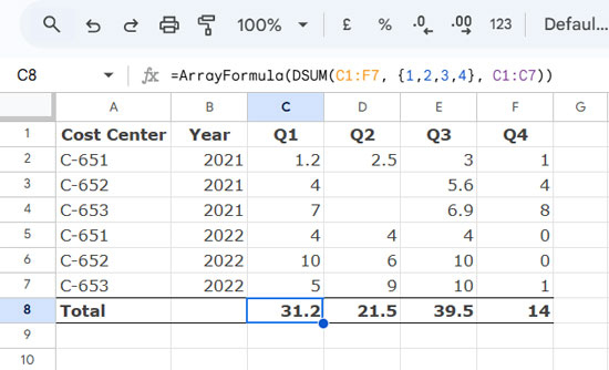
Why Move Away from Database Functions?
While database functions work well for aggregation and lookup, they have limitations. If you wanted to apply a SPARKLINE or FORMULATEXT formula to each column, you would have had to manually drag the formula across columns. Additionally, database functions require structured data, which may not always be ideal.
This is where the BYCOL function in Google Sheets fills the gap, allowing you to apply custom formulas to each column dynamically.
BYCOL Function Syntax and Arguments
Syntax:
BYCOL(array_or_range, lambda)Arguments:
- array_or_range – The array or range processed column by column.
- lambda – A custom unnamed LAMBDA function applied to each column.
LAMBDA Syntax:
=LAMBDA(name, formula_expression)Step-by-Step Guide: Using the BYCOL Function in Google Sheets
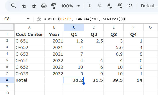
Let’s replace the DSUM formula from earlier with BYCOL and LAMBDA.
Steps:
- Use a regular formula to total a column:
=SUM(C2:C7) - Convert it into a custom LAMBDA function:
=LAMBDA(col, SUM(col))Here,colis the assigned name for each column. - Apply BYCOL to process all columns at once:
=BYCOL(C2:F7, LAMBDA(col, SUM(col)))
Now, instead of manually dragging formulas, BYCOL automates the process dynamically.
BYCOL Function Examples
Here are more cases of use for the BYCOL function in Google Sheets.
1. COUNTIF for Each Column
Count values greater than 5 for each column:
=BYCOL(C2:F7, LAMBDA(col, COUNTIF(col, ">5")))2. COUNTIFS for Each Column
Count values greater than 2 and less than 4:
=BYCOL(C2:F7, LAMBDA(col, COUNTIFS(col, ">2", col, "<4")))3. Expanding SPARKLINE Results with BYCOL
Generate a column chart for each quarter’s sales:
=BYCOL(C2:F7, LAMBDA(col, SPARKLINE(col, {"charttype", "column"; "max", 30; "color", "red"; "empty", "zero"})))Do I Need ARRAYFORMULA with BYCOL?
You may encounter #VALUE errors when using BYCOL in Google Sheets. If the error message states “An array value could not be found,” you likely need ARRAYFORMULA.
Example: Counting Blank Cells with ARRAYFORMULA
=ArrayFormula(BYCOL(C2:F7, LAMBDA(c, SUM(--(ISBLANK(c))))))This formula counts blank cells in each column of C2:F7 and returns an array result like {0,1,0,0}.
Key Takeaways
- The BYCOL function in Google Sheets automates column-wise calculations.
- It simplifies repetitive formulas and eliminates the need for dragging across columns.
- Works best for SUM, COUNTIF, SPARKLINE, and other column-wise functions.
- If you face #VALUE errors, use ARRAYFORMULA for array-dependent functions.