These days, it’s easy to search for a value in an entire table and return the column header in Google Sheets. Modern formulas using functions like BYCOL, MATCH, or XMATCH make this possible. But even before that, we had a clever and simpler formula that combines SEARCH, SORTN, and HLOOKUP.

In this tutorial, you’ll learn how to use this older—but still powerful—approach and how it compares to the modern method.

How Searching an Entire Table and Returning the Header Works

I have employees working in the Northern, Southern, Eastern, and Western regions. In my Google Sheet, the regions are listed in cells B2:E2, and the corresponding employees are listed below each region.

Goal: Look up an employee’s name and return the region they work in.

This is exactly what we mean when we say “search a value across a table and return the header in Google Sheets.”

Default Behavior of HLOOKUP

As you may know, HLOOKUP is designed to search across the first row of a table and return a value from a specified row index within the column where the match is found.

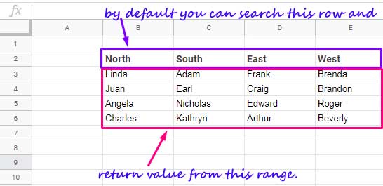
You can look up a region name like “South” using HLOOKUP, since region headers are in the first row of the table:

=HLOOKUP("South", B2:E, 2, 0)

This formula returns “Adam”, assuming “South” is in C2 and “Adam” is in C3.

HLOOKUP Hack: Search the Entire Table and Return the Header

Now let’s look at the HLOOKUP formula that searches through the entire table and returns the header of the column where the match is found.

=HLOOKUP(1, {SORTN(SIGN(SEARCH(F3, B3:E))); B2:E2}, 2, 0)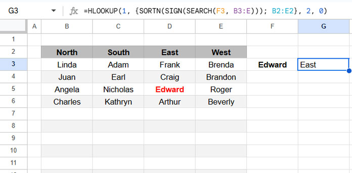

What It Does:

• F3 = cell containing the lookup value
• B3:E = the table data (excluding headers)
• B2:E2 = the header row

This formula returns the header of the first matching column based on a partial match of the value in F3.

Note: This method only returns the first match. If you want to return all matching headers, check out my other tutorial:
Search Across Columns and Return the Header in Google Sheets (using BYCOL + XMATCH)

Formula Breakdown

Syntax: HLOOKUP(search_key, range, index, [is_sorted])

In this case:

• search_key = 1
• range = {SORTN(SIGN(SEARCH(F3, B3:E))); B2:E2}
• index = 2
• is_sorted = 0 (for exact match)

Let’s break down the range part:

Step-by-Step:

SEARCH(F3, B3:E)

Searches for the value in F3 across the range B3:E. Returns an array of positions or #VALUE! errors.

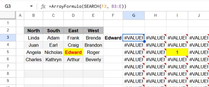
SIGN(SEARCH(F3, B3:E))

Converts numeric positions to 1 and errors to 0. This gives a binary row where 1 means a match.

SORTN(...)

Returns only the first 1 in the row (i.e., first match). Ensures only one column is picked.

{SORTN(...); B2:E2}

Combines this row with the header row to form a lookup table for HLOOKUP.

Case-Sensitive Match

The formula above uses SEARCH, which is case-insensitive.

If you want a case-sensitive version, replace SEARCH with FIND:

=HLOOKUP(1, {SORTN(SIGN(FIND(F3, B3:E))); B2:E2}, 2, 0)

Important Notes

• SEARCH and FIND both perform partial matches.
  • They behave like "*key*" (i.e., the value appears anywhere in the cell).
• If you want to match only values that start with the key (like "key*"), you’ll need to customize the logic accordingly—simply remove the SIGN function from the formula.
• This is not an exact-match method. If you need exact matches, consider switching to the modern BYCOL + XMATCH method.

Related Resources

Here are more tutorials to help you work with headers and lookup functions in Google Sheets:

• Find Max N Values in a Row and Return Headers
• Lookup Header and Filter Non-Blanks
• Find the Column Header of the Max Value
• Find the Column Header of the Min Value
• Get the Headers of the First Non-Blank Cell in Each Row
• Get the Header of the Last Non-Blank Cell in a Row