In this tutorial, we’ll see how to use conditional formatting to highlight the latest value/status change rows in Google Sheets.

I have an employee database in Sheets that tracks job titles.

For example, take employee Ben:

• He joined in January as an Engineer.
• Later, in May, his designation changed to Manager.
• After that, there were no more changes.

So the latest value change for Ben is in May. That’s the row I want to highlight.

I have already posted a tutorial on how to filter the last status change rows. You can check that here – Google Sheets: Show Only the Last Status Change per Name.

Here, instead of filtering, we’ll use highlighting.

Sample Data

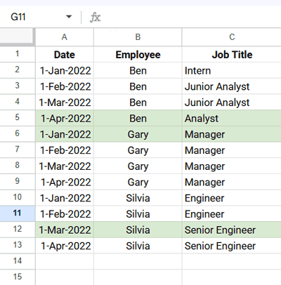
We have the following data in A1:C:

Column C is where the values change.

👉 Important: Your data should be sorted first by Date, then by Employee.
This way, the formula can correctly identify the latest status change rows.

• Ben: last change → 1-Apr-2022
• Gary: no changes → highlight the first row (1-Jan-2022)
• Silvia: last change → 1-Mar-2022

👉 Edge case: If an employee goes Engineer → Senior Engineer → Engineer, the formula will highlight the first Engineer row, not the last one. Rare case, but good to know.

Google Sheets Conditional Formatting Formula

We need a custom formula for this:

=AND(
  $B2<>"", 
  ROW($B2)=
    ARRAYFORMULA(
      XLOOKUP(
        $B2 & XLOOKUP($B2, $B$2:$B, $C$2:$C, , 0, -1), 
        $B$2:$B & $C$2:$C, 
        ROW($B$2:$B)
      )
    )
)

In Google Sheets, this helps you track the date when each employee’s latest status change began.

Steps to Apply Conditional Formatting

1. Select your dataset (A2:C).
2. Go to Format → Conditional Formatting.
3. Under Format rules, pick Custom formula is.
4. Paste the above formula.
5. Choose a highlight color.
6. Done.

Now the latest change rows are highlighted automatically.

Formula Explanation

• The inner XLOOKUP looks from bottom to top and fetches the latest job title for each employee.
• The outer XLOOKUP returns the row number of that match.
• ARRAYFORMULA is necessary here because we’re combining arrays (Employee&JobTitle) and need the formula to handle multiple rows at once.
• AND($B2<>"", …) just avoids blank rows.

Example:
Take Silvia. Her job titles are:

• Jan → Engineer
• Feb → Engineer
• Mar → Senior Engineer
• Apr → Senior Engineer

The inner XLOOKUP (bottom-to-top) finds Senior Engineer as Silvia’s latest role.
The outer XLOOKUP (top-to-bottom) then returns the row number of the first occurrence of Senior Engineer for Silvia (i.e., the row on Mar 1).
That’s why the formula highlights Silvia’s Mar 1 record — her last status change.

So, the formula highlights the row where the last value change for each employee is recorded.

Sample Sheet

You can make a copy of the sample sheet I used in this tutorial.

Copy Sample Sheet

Note: The sheet also contains formulas from my previous tutorial on filtering the latest status change rows. You can safely ignore them while testing the highlighting rule.

Related Resources

• Lookup Latest Value in Excel and Google Sheets
• How to Lookup Latest Dates in Google Sheets
• Retrieve the Earliest or Latest Entry Per Category in Google Sheets
• Combine Rows and Keep Latest Values in Google Sheets
• Get the Latest Non-Blank Value by Date in Google Sheets