


")


")

")
")
 in Excel & Google Sheets")


The easiest way to compare two lists and highlight matches or differences is by using the XMATCH function in Google Sheets.
To highlight matches, you can use the following formula:
=XMATCH(lookup_value, lookup_array)To highlight mismatches, use the following formula:
=AND(lookup_value<>"", NOT(IFNA(XMATCH(lookup_value, lookup_array))))Where:
lookup_valueis the relative reference to the starting cell of the first list you want to compare.lookup_arrayis the absolute range reference of the array you want to compare to.
Examples
Highlight Matches in Two Lists in Google Sheets
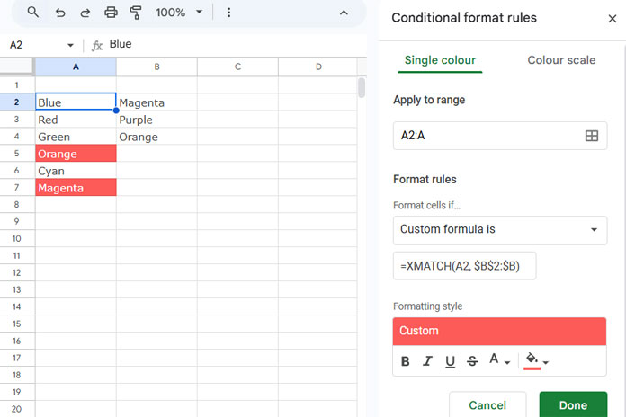
Let’s assume you want to compare the lists in A2:A and B2:B and highlight the matches in A2:A.
Follow these steps:
- Select the range
A2:A(the range you want to highlight). - Click on Format > Conditional Formatting.
- Under Format cells if, select Custom formula is.
- In the formula field, enter:
=XMATCH(A2, $B$2:$B)- Choose a formatting style and click Done.
This formula compares each value in A2:A with the values in B2:B and highlights the matching values.
This method is useful when, for example, you have two groups of students and want to identify those in the first group accidentally included in the second group.
The XMATCH function checks each value in list 1 (column A) against list 2 (column B) and returns a number (the relative position in list 2) if a match is found. If no match is found, it returns an #N/A error. This results in highlighted cells wherever the formula returns a number.
Highlight Differences in Two Lists in Google Sheets
Highlighting differences is straightforward. You just need to highlight cells where the formula returns an #N/A error. To do this, follow these steps:
- Wrap the formula with IFNA to replace
#N/Awith an empty string:
IFNA(XMATCH(A2, $B$2:$B))- Wrap it with NOT to return
TRUEfor empty cells andFALSEfor matches:
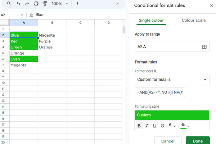
NOT(IFNA(XMATCH(A2, $B$2:$B)))This formula will highlight all differences in list 1. However, it may also highlight empty cells, which you likely don’t want. To exclude empty cells, use AND as follows:
=AND(A2<>"", NOT(IFNA(XMATCH(A2, $B$2:$B))))You can use this formula to highlight mismatched values in A2:A.
The process for applying this rule is the same as for highlighting matches. You just need to replace the formula in the Conditional Formatting panel with the one for highlighting differences.
What to Do When the Lists are in Two Different Sheets within a Workbook?
When highlighting matches or differences with the above formulas in one sheet, you won’t encounter any issues. However, when list 1 is in one sheet and list 2 is in another sheet, you need to adjust the formula.
In conditional formatting, when referring to a different sheet, you must use the INDIRECT function.
For example, assume list 1 is in Sheet1!A2:A and list 2 is in Sheet2!B2:B. The formulas (highlight rules) will be:
Highlight Matches:
=XMATCH(A2, INDIRECT("Sheet2!B2:B"))Highlight Differences:
=AND(A2<>"", NOT(IFNA(XMATCH(A2, INDIRECT("Sheet2!B2:B")))))
Hi, Prashanth,
Thank you for making life easy.
Can you tell me the syntax for adding three or more sheets to-
=ArrayFormula(countif(indirect("Sheet2!$B$2:$B"),$A2:$A))>0Hi, AJ,
I’m not clear. Do you want to compare more than two lists (in different sheets in a file) and find the matches in all of them?
Hi Prashanth,
Is there a way to generate a “List3” based on the unique items combined from List1 and List2?
Many thanks!
Hi, Vivian,
Formula based on my lists in columns A and B.
=Query(unique({A2:A;B2:B}),"Select * where Col1 is not null")Best,
So let’s say I have multiple tabs of information and I want to do a match that searches multiple tabs. i.e.= If I type “XX” into either Tab 1, Tab 2, or Tab 3 it will search Tab 4, Tab 5, and Tab 6 for a match. If it finds a match, it will highlight the match in Tab 4, Tab 5, or Tab 6.
Hi, Kim,
Instead of giving you a specific answer, I wish to bring your attention to my following tutorials.
1. Compare Two Google Sheets Cell by Cell and Highlight.
2. How to Conditional Format Duplicates Across Sheet Tabs in Google Sheets.
Best,