


")


")

")
")
 in Excel & Google Sheets")


I’ll deviate from traditional approaches to highlight the largest 3 (or N) values in each row in Google Sheets. The common methods using LARGE and RANK have unpredictable issues that can lead to incorrect results. What are they?
The Problem with Traditional Methods
We usually use the LARGE function to find the nth largest value. In conditional formatting, it helps highlight the top 3 values in a row. However, this approach has some issues:
- Empty Cells Cause Errors: If most of the row’s cells are empty, LARGE may return a
#NUM!error. To fix this, you can use the N function to return0for empty cells. But improper usage can lead to incorrect highlighting. - Ties in the Top 3: The RANK function (or LARGE + N) is often preferred to handle ties. However, it automatically includes all occurrences of the nth largest value. This means if multiple values tie for the third-highest spot, all of them will be highlighted, exceeding the limit of 3 highlights.
Example: Unexpected Extra Highlights Due to Ties
Assume a row contains the numbers: 30, 20, 20, 20, 10, 10, 5. The third-largest value is 20, but because there are three occurrences of 20, all of them get highlighted.
| Score | 30 | 20 | 20 | 20 | 10 | 10 | 5 |
| Rank | 1 | 2 | 2 | 2 | 5 | 5 | 7 |
This means the top 3 + all duplicates of the 3rd value get highlighted, not just the top 3. So, handling ties properly is crucial when you highlight the largest 3 values in each row.
4 Approaches to Highlight the Largest 3 Values in Each Row
To handle ties effectively, I’ve developed four formulas to highlight the top 3 values in each row. Choose the one that best fits your needs:
| Values | 1. Top 3 (Exactly 3, No Extra Ties) | 2. Top 3 + All Duplicates of Nth | 3. Top 3 (Distinct Values Only) | 4. Top 3 (Distinct Values + All Occurrences) |
| 30 | ✅ | ✅ | ✅ | ✅ |
| 20 | ✅ | ✅ | ✅ | ✅ |
| 20 | ✅ | ✅ | ☑️ | |
| 20 | ☑️ | ☑️ | ||
| 10 | ✅ | ✅ | ||
| 10 | ☑️ | |||
| 5 |
How These Methods Differ:
- First & Third Methods: Highlight exactly 3 values (first method includes ties, third method ensures uniqueness).
- Second Method: Highlights top 3 including duplicates of the nth value.
- Fourth Method: Highlights top 3 distinct values + all occurrences of those values (duplicates in a separate color for clarity).
Example Formulas for Highlighting Top 3 in Each Row
1. Top 3 (Exactly 3, No Extra Ties)
This formula highlights exactly 3 values, ignoring extra ties:
=AND(B2<>"", XMATCH(CELL("ADDRESS", B2), SORTN(TOCOL(ADDRESS(ROW($B2:$K2), COLUMN($B2:$K2))), 3, 0, TOCOL($B2:$K2), FALSE)))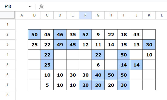
Steps to Apply in Google Sheets:
- Select the range where you want to apply the rule (e.g., B2:K7).
- Click Format > Conditional formatting.
- In the Format Rules section, select Custom formula is.
- Enter the formula.
- Choose a formatting style (e.g., bold text, background color).
- Click Done.
How It Works:
- SORTN selects the address of the top 3 largest values in each row.
- XMATCH checks if each cell’s address appears in the sorted list.
B2<>""ensures that empty cells are ignored.
2. Top 3 + All Duplicates of Nth
This formula highlights top 3 + all duplicates of the 3rd value:
=RANK(B2, $B2:$K2)<=3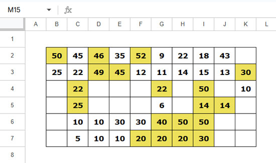
- How It Works: If a number ranks ≤3, it gets highlighted, including all duplicates of the 3rd highest value.
3. Top 3 (Distinct Values Only)
To highlight only 3 unique top values:
=AND(XMATCH(B2, SORTN(TOCOL($B2:$K2, 3), 3, 2, 1, FALSE)), COUNTIF($B2:B2, B2)<2)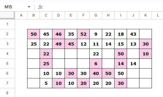
- XMATCH matches each value in the top 3 largest unique values returned by SORTN.
- COUNTIF ensures only the first occurrence of each value is highlighted.
4. Top 3 (Distinct Values + All Occurrences)
To highlight top 3 unique values and all duplicates separately:
=XMATCH(B2, SORTN(TOCOL($B2:$K2, 3), 3, 2, 1, FALSE))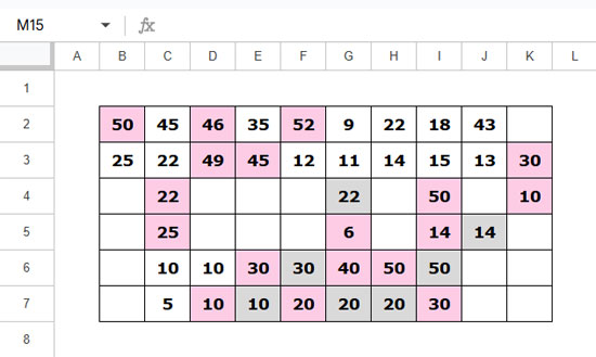
- Use this rule as a second rule alongside the previous one and apply a different color to distinguish duplicates.
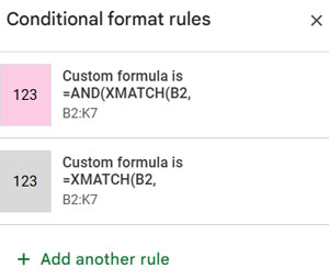
- This formula is the same as the previous one except it does not use COUNTIF, meaning it highlights all occurrences of the top 3 unique values instead of just the first.
Real-Life Applications of These 4 Approaches
| Approach | Where It’s Useful |
| Top 3 (Exactly 3, No Extra Ties) | Competitions, business reports, funding allocation. |
| Top 3 + All Duplicates of Nth | Leaderboards, performance reviews, sales rankings. |
| Top 3 (Distinct Values Only) | Pricing strategies, salary bands, data summaries. |
| Top 3 (Distinct Values + All Occurrences) | HR & rewards, market research, visualizing tied results. |
Conclusion
The traditional LARGE and RANK methods have limitations, especially when handling ties. With these four improved formulas, you can highlight the largest 3 values in each row in Google Sheets while controlling tie behavior according to your needs.
By selecting the right formula, you ensure that your data visualization is both accurate and meaningful.
Can you do this for a single column: highlight three largest values in a column? TIA
Hi, Chris,
The same formula will work in a vertical range.
For example, for the range C2:C15, you can use the following highlight rule.
=and(len($C$2:$C$15),C2>=large(arrayformula(n($C$2:$C$15)),3))Hello,
Is there a way to do this but not highlight a duplicate lower value? For instance, if my values are 50, 49, 48, 48, 40, and 30, I would only want 50, 49, and the first 48 highlighted, not both 48s.
Thank you.
Hi, Mark K,
I have already posted the highlighting rules for that. You can find that HERE.