


This tutorial includes two conditional formatting rules to highlight groups when the group total exceeds target in Google Sheets.
Are you using Google Sheets to record your sales or procurement details? Then there will be multiple rows with the same items called groups.
In such data, with conditional formatting, you can test whether the total sales or procurements meet the target.
You can get group totals in Google Sheets by using the function Sumif. If you want to include some conditions before totaling the group, then you can use Sumifs or Query.
What about conditionally highlighting groups that based on group totals?
This post contains two custom conditional formatting formulas that you can use to highlight groups when group total exceeds target in Google Sheets. No doubt, the function Sumif will be the key in those rules.
I have included two types for formulas keeping in mind your data formatting. Your data may not be arranged as per my sample data below. So, I hope, giving two options will give you some flexibility.
Sheets Formula to Highlight Groups When Group Total Exceeds Target
I have two real-life examples (to include the above said two options).
- Highlight rows when monthly allocation percentage exceeds the target.
- Conditional format when total sales meet the target.
Highlight Rows When Monthly Allocation Exceeds Target in Google Sheets
I have a sample campaign data in Google Sheets that starts with a Campaign column, then followed by Total Budget, and Monthly Allocation (please see the following image).
Add a fourth column to this data range titled “Allocation Percentage”. In that, in cell D2 enter the following formula.
=ArrayFormula(if(len(B2:B),C2:C/B2:B,))Then format D2:D to Percent from the menu Format > Number > Percent.
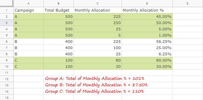
Here my below conditional formatting formula highlights group A and C since the total monthly allocation percentage of these groups are exceeding 100%.
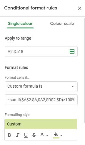
Here is that Sumif based custom formula rule. How to apply this rule? I’ll come to that later.
=sumif($A$2:$A,$A2,$D$2:$D)>100%To understand the highlighting rule, just sum the ‘Monthly Allocation %’ of group A as below.
=sum(D2:D)The result would be 101%. That means here the group total exceeds the target.
In the above Sumif formula, the range is ‘Campaign’ (group) and the sum_range (the column to total) is the ‘Monthly Allocation %’. The criterion in the formula is the ‘Campaign’ name.
The rule tests whether the group-wise ‘Monthly Allocation %’ (Sumif output) is greater than 100%.
Referring to the Sumif syntax below will be helpful to you to understand the arguments and the corresponding range, criterion, and sum_range used in my Sumif formula.
SUMIF(range, criterion, [sum_range])How to apply the above Sumif formula in conditional formatting to highlight rows based on group totals in Google Sheets?
Steps:
- Click on the cell A2.
- Go to Format > Conditional formatting.
- Apply the below settings.
This formula highlights the entire row in the range. For example, A2:D5 in the first group instead of A2:A5.
To limit that highlighting to a single column, remove the dollar sign in the criterion reference in the formula. Then the formula will be as follows.
=sumif($A$2:$A,A2,$D$2:$D)>100%You May Like: Sumif in Conditional Formatting in Google Sheets.
Conditional Format Rows When Total Sales Meet Target
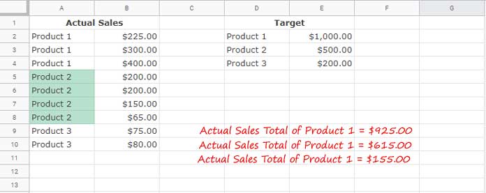
Here first see the sample data. As you can see the data format is entirely different when compared to the previous example.
Let’s leave the data formatting part and concentrate on the highlighting of cells.
As per the provided data, here only the product 2 meets the target. Just sum the range B5:B8 to check the total.
=sum(B5:B8)You will get $615.00 as the result of the above formula. That total is greater than our sales target of Product 2, which is $500.00 (cell E3). So in this case, the total sales meet the target.
Check the other two products and you can see that both of them do not meet the set target.
Create Custom Rule to Highlight Groups When Sales Total Exceeds Target in Google Sheets
Similar to the first example, here also we want to highlight the rows when a group total exceeds the target. But one thing is different here. That is the data formatting.
You can use the same Sumif formula (with adjusting range, criterion, and sum_range) if you can re-arrange the data as below.
Formula:
=sumif($A$2:$A,A2,$C$2:$C)>B2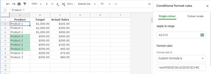
Here instead of using >100% which is the target in the first formula, use >B2 which is the target here.
But some of you may want to preserve the data formatting, right? I mean the actual sales in A1:B and target in D1:E.
In such a case, we can use Vlookup with Sumif as combo formula.
=vlookup(A2,$D$2:$E$4,2,0)<sumif($A$2:$B$10,A2,$B$2:$B$10)Formula Explanation:
Here to conditional format the products based on their sales volume and target, we can use the Sumif as in earlier examples. But additionally, we may depend on Vlookup.
While the Sumif formula sums the sales amount (column B), the Vlookup returns the corresponding target value from column E.
The formula checks the rows like this.
For the first product;
Product 1 Target (E1) < to sum of Product 2 Sales (B2:B4)Which is equal to =1000<925 which would return FALSE.
Here the Product 1 Target (E2) is returned by the Vlookup and the sum of Product 1 Sales (B2:B4) is returned by the Sumif.
That means the formula tests whether the target value is less than the total sales. If the formula returns TRUE, such groups got highlighted.