I am providing you with 10 custom Google Spreadsheet formulas that I believe will be useful for you to ease your day-to-day office tasks.
If you have only the basic know-how of Google Sheets, you will definitely find these custom Google Sheets formulas useful.
You can use it straightway by following the tips without even knowing the code/function in use.
Is There Any Free Guide to Learn Google Spreadsheet Formulas?
Of course, you can find many of them online and that may be free/paid. But I have around 500 plus formulas under the tag Spreadsheet on this site. All are unlocked and no sign-up or subscription is required to access!
In addition to that, I have covered most of the functions in Google Sheets with simple and easy to follow examples. There is a Google Sheets functions’ Index to help you quickly navigate through the functions.
In this tutorial, I am sharing you with the 10 most useful Google Spreadsheets formulas.
Row Google Spreadsheet Formula for Auto Row Numbering
As you may have seen, serial number column is part of many of the official formats. In your office also you have seen or using formats starting with serial numbers.
You can automate this in Google Spreadsheet with one custom formula.
=ArrayFormula(row(A1:A20))
This formula would populate the numbers from 1 to 20 in sequential. Just apply this in any cell. You can see the numbers 1 to 20 populates in that column downwards.
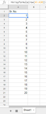
Change the cell reference A20 in the formula to the number that you want. If you put 50 the numbering will be from 1 to 50.
If you see the error #REF! don’t get panic! It says;
Array result was not expanded because it would overwrite data in …
The reason there are not enough blank cells for this formula to populate. So make sure that the cells are blank below.
Find More Detail on this Topic: Auto Serial Numbering in Google Sheets with Row Function
Google Spreadsheet Formula to Match Two columns to Find the Difference
This is another common task in office, i.e. compare or match two lists.
Example:
I had prepared a list of vegetables and then placed the order with a vendor – This is my ‘List 1’.
Later I have received the ordered items – List 2.
How do I check whether all the ordered items are received?
If both the lists are in same alphabetical order or item wise, you can compare it side by side. But it may or may not be in such order.
Here is my custom Google Spreadsheet formula to compare or match two lists. It works well with your list. It doesn’t matter how the items are arranged in the two lists.
=ArrayFormula(if(iferror(match(A2:A10,B2:B10,0))="","Not Found","Found"))
Change the range A10 and B10 to the last cell in your list.
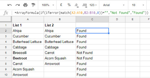
In this custom Google Spreadsheet formula, I have used the function Match. There is a different solution using REGEX – Match Two Columns that Contain Values Not in Any Order Using Regex.
The Killer Google Sheets Formula to Calculate Net Working Days that Excluding Weekends and Official Holidays
Are you working in HR/ADMIN/Accounts?
The following formula can help you to make an error-free final settlement of your employees. Also, it can definitely save your couple of minutes time.
How to Calculate the Networking Hours of Employees?
Here I am going to use the NETWORKDAYS.INTL function. What you want to do is;
Enter the start date (employee joining date) in one cell (A2) and the end date (employee leaving date) in another cell (B2).
In the next column (Column C) enter the list of your official holidays during that period. If you want, you can even include the absent days of the employee in the holiday list.
Formula:
=NETWORKDAYS.INTL(A2,B2,1,C2:C15)
Example:
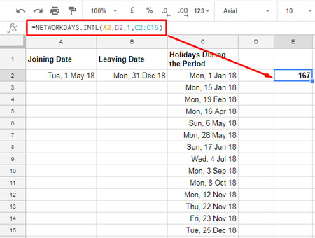
In this formula, the weekends are SATURDAY/SUNDAY. The 1 in the formula indicates this. I know your weekends may be different. You can pick your desired weekend number from the below list.
2 = Sunday/Monday, 3 = Monday/Tuesday, 4 = Tuesday/Wednesday, 5 = Wednesday/Thursday, 6 = Thursday/Friday, 7 = Friday/Saturday.
11 = Sunday, 12 = Monday, 13 = Tuesday, 14 = Wednesday, 15 = Thursday, 16 = Friday, 17 = Saturday
Must Read: Learn the complete date related functions in Google Sheets.
Custom Google Sheets Formula to Calculate Normal/Over Time Hours
Here is one ‘versatile’ formula to calculate the hours between a start time and end time in Google Sheets.
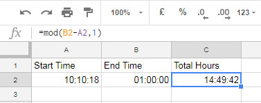
Here are the two common questions that I am expecting from you about the above formula.
- What is the peculiarity of this formula?
2. Why don’t you simply use end time – start time to get the time difference?
Here is my answer. My work start time and work end times are on two different days.
You can use the end time – start time approach only if the times are recorded on the same day or your entered time is in the date time (timestamp) format.
Start Time (in Cell A1): 10:10:18
End Time (in Cell B1): 16:10:18
Here you can follow the normal Google Spreadsheet formula like;
=B1-A1
But I highly recommend you to use the below Google Spreadsheet formula that using the MOD function as it can correctly calculate the time difference.
=mod(B1-A1,1)
Needless to say, this is a killer time calculation formula.
Here you can find more details – Google Sheets: The Best Overtime Calculation Formula.
Google Spreadsheet Formula to Generate a Full Month’s Dates in a Row/Column
Enter the year (in number format) in Cell A1 and the month (text format) in Cell A2.
In Cell A2, enter the month in a text format that also in three characters long.
For example “Jan” for January, “Feb” for February etc. Rest the formula will take care of.
Formula:
=ArrayFormula(TRANSPOSE(TO_DATE(row(indirect(date($A$1,month($A$2&1),1)&":"&eomonth(date($A$1,month($A$2&1),1),))))))
Example:

Related Topic: Populate a Full Month’s Dates Based on a Drop-down in Google Sheets.
SORTN Google Sheets Function to Find Top N Rank Holders
Ever used the function SORTN in Google Sheets? It’s a beast!
The function SORTN is of course for sorting your data. But there are a lot more hidden behind.
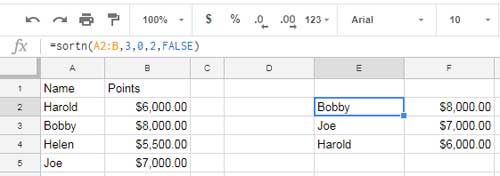
Here see how to find the top N rank holders using a SORTN formula.
For this test, my column A contains the name of participants and column B contains their points/scores.
=sortn(A2:B,3,0,2,FALSE)
This formula would return the top 3 rank holders. Change the number 3 to the number that you want.
For example, change 3 to 2 to get the top 2 rank holders.
Similar: How to Use SORTN Function in Google Sheets to Extract Sorted N Rows
GoogleFinance Formula to Convert Currency
I want to convert my local currency to US Dollar. How to do that? The answer is the function GoogleFinance.
The below Google Spreadsheet formula would provide you with the USD to INR exchange rate. That means 1 USD = how much INR?
=GoogleFinance("CURRENCY:USDINR")
For other currencies and more details follow my tutorial – How to Convert Currency in Google Sheets Using GoogleFinance Function.
Google Sheets Query Formula to Group/Summarise a Date Column in Month/Year Wise
All the Spreadsheet users should know at least one method to make a summary of the data in hand.
Here is a custom formula to help you make a summary of date column.
Use the below formula if your Column A contains dates and Column B contain numbers.
Google Sheets Formula to Do a Month Wise Summary:
=query(A1:B8,"Select Month(A)+1,Sum(B) group by month(A)+1")
Google Sheets Formula to Do a Year Wise Summary:
=query(A1:B8,"Select Year(A),Sum(B) group by Year(A)")
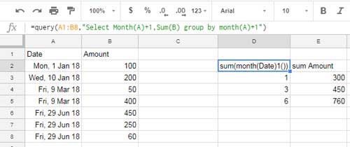
Learn in Detail: Filter by Month and Year in Query in Google Sheets.
Formula Based Search in Google Spreadsheet Using Vlookup
Normally the first column in our spreadsheet data may contain product ID, names, descriptions, dates, month name etc.
Using the Vlookup formula, you can search in that column and if found the search key, return a value from the row found.
Here is one custom Vlookup formula for you to use.
=vlookup("March",A1:B13,2,FALSE)
Result: 5500.00
In this “March” is the search key.
A1:B13 is the range to search.
In that, the formula would only search the key in A1:A13, the first column.
The formula returns the value from the second column.
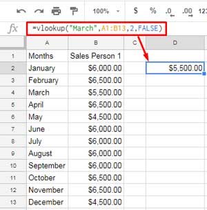
Must Check: Vlookup in Google Sheets – 10 Formula Variations, Tips, and Tricks.
IMPORTRANGE: Custom Formula to Connect Two Google Sheets
How to import content from Spreadsheet A to Spreadsheet B? The answer is IMPORTRANGE.
How?
Just grab the URL of the Spreadsheet A and use it in the IMPORTRANGE formula in Spreadsheet B as below.
=importrange("https://docs.google.com/spreadsheets/d/17Wh7kenRWRMZmbKGoZOVkNsX-3hM5eHuv-InZ02_2gc/edit#gid=1100774393","Sheet1!A1:B")
The last part of the formula is the data range to import. In that range Sheet1 is the tab name in Spreadsheet A and A1:B is the range to import.
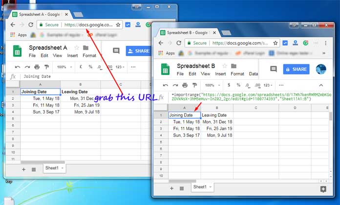
Any future changes in the rangeSheet1!A1:B will be reflected in Spreadsheet B.
Hope you may find the above 10 custom Google Spreadsheet formulas useful. Any query, do write to me in the comments.
