Google Sheets ISODD Function – Formula Examples

The odd number returns a reminder when divided it by # 2. Google Sheets ISODD function helps you to identify such numbers. Examples to odd numbers are 1, 3, 5 and so on.

Google Sheets ISODD function will return TRUE (Boolean value) if the number tested is odd. If the number is not odd (even), no doubt, the function will return FALSE (Boolean value).

This TRUE/FALSE Boolean values generally used in conditional statements that involve the IF Logical function. I’ll explain that later.

Other than identifying the odd numbers in Sheets, this function can be useful in conditional formatting, filtering rows, data validation (see the additional resource section at the bottom), etc.

In this Google Spreadsheet tutorial, I have included some formula examples to the use of the ISODD function.

Syntax of the ISODD Function in Google Sheets

Syntax:

ISODD(value)

Example:

=isodd(3)

If the value is in a cell, the formula can be used as below.

=isodd(A1)

To use multiple values in ISODD, use it together with the ArrayFormula function.

ISODD Array Formula Syntax:

=ArrayFormula(isodd({value1,value2,value3...}))

Example:

=ArrayFormula(isodd({12,3,4,59}))

If the values are in an array, then the formula will be as below.

=ArrayFormula(isodd(A1:A5))

Formula Examples to Google Sheets ISODD Function

You can use numbers, date and time as the ‘value’ arguments in Google Sheets ISODD function. If you input a text string, the formula would return a #VALUE! error.

Basic to Google Sheets ISODD function

See the numbers in cell A3, A4, and A5. The formula reads that numbers like 1, 1, and 2 respectively as this function truncates the decimal.

If you use the below formula, the output would be FALSE as 0 (zero) is an even number.

=isodd(0)

Remove all the formulas in the array B2:B12 and then key in this array formula in cell B2.

=ArrayFormula(isodd(A2:A12))

This ISODD array formula will test the vales in multiple rows and expand the result accordingly.

ISODD With IF Logical Test in Google Sheets

In some countries, the odd numbers as considered as sacred. Here is a simple logical test based on this.

Assume 92756 is your vehicle registration number. You want to total the number of digits in this registration number and test whether it is odd or even.

I mean the total of;

=9+2+7+5+6

Here is the formula to split and sum the digits.

=sum(split(regexreplace("92756", "(.{1})", "$1,"),","))

The above SPLIT + REGEXREPLACE combo will split and sum the digits given on the number plate.

You May Like: Split Number to Digits in Google Sheets.

Enclose the above formula within ISODD and then use that in a logical test.

=if(isodd(sum(split(regexreplace("92756", "(.{1})", "$1,"),",")))=TRUE,"LUCKY","UNLUCKY")

The above formula would return the string “LUCKY” if the total of the number of digits is an odd number, else “UNLUCKY”

Filter Odd Rows

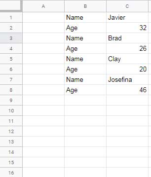
Google Sheets ISODD function can be useful to Filter data. Assume your data entry operator is new in his business. See how he had entered the data. You want the name in one column and age in another. How to format this data properly?

Filter every alternate odd rows in Sheets

See how I am filtering out the age and extract the names only, using an ISODD formula in Sheets.

=ArrayFormula(filter(B1:C8,isodd(row(B1:C8))))

Sometimes you may need to replace the ISODD with ISEVEN depending on the starting row number.

ISODD in Conditional Formatting in Sheets

Google Sheets offers a built-in rule to highlight alternate rows. That’s available under the Format menu.

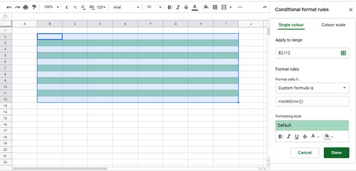
You can also use the ISODD function to highlight every alternate row. How?

  1. Select the range to highlight. As an example, here I am going to select the range B2:I12.
  2. Go to Format > Conditional formatting.
  3. Enter the below formula in the provided field under the “Custom formula is” drop-down.
=isodd(row())
Highlight every alternate columns and rows

You can also use the ISODD function to highlight every alternate column.

Keep the above range selected. Just change the above formula. I mean use the below ISODD formula with the value as the current column number.

=isodd(column())

Additional Resources:

  1. How to Use ODD Function in Google Sheets.
  2. How to Generate Odd or Even Random Numbers in Google Sheets.
  3. The Best Data Validation Examples in Google Sheets (included the role of ISODD in data validation).
  4. How to Move Values in Every Alternate Row to Columns in Google Sheets.
  5. How to Use EVEN Function in Google Sheets.
Prashanth KV
Prashanth KV
Your Trusted Google Sheets and Excel Guide Prashanth KV brings a wealth of experience in Google Sheets and Excel, cultivated through years of work with multinational corporations in Mumbai and Dubai. As a recognized Google Product Expert in Docs Editors, Prashanth shares his expertise through insightful blogging since 2012. Explore his blog for practical tips and guidance on maximizing your spreadsheet skills.

Hierarchical Numbering Sequences in Excel

Creating hierarchical numbering sequences in an Excel spreadsheet can significantly improve the way you...

How to Easily Repeat a Sequence of Numbers in Excel

Excel offers multiple ways to accomplish tasks, and the simplicity of each approach depends...

Create a Sequence of Dates at Every Nth Row in Excel (Dynamic Array)

Would you like to create a sequence of dates in every nth row in...

XMATCH Row by Row: Finding Values Across a Range in Google Sheets

Using the BYROW function with XMATCH in Google Sheets allows us to match values...

More like this

XMATCH Row by Row: Finding Values Across a Range in Google Sheets

Using the BYROW function with XMATCH in Google Sheets allows us to match values...

Limit Formula Expansion to a Specific Row in Google Sheets

In this tutorial, I’ll explain how to limit the expansion of an array formula...

3-D Referencing Structured Data Tables in Google Sheets

When you have several tables within a single sheet—not across multiple sheets in a...

LEAVE A REPLY

Please enter your comment!
Please enter your name here

This site uses Akismet to reduce spam. Learn how your comment data is processed.