How to Use the ISODD Function in Google Sheets (With Examples)

The ISODD function in Google Sheets checks whether a number is odd. It returns TRUE if the number is odd and FALSE if it’s even. This makes it useful for logical formulas, conditional formatting, filtering alternate rows or columns, and more.

In this tutorial, you’ll learn how to use the ISODD function with practical examples and variations.

Table of Contents

Syntax of ISODD

ISODD(value)

value: A number, cell reference, or expression to test for oddness.

Examples:

=ISODD(3)   // TRUE
=ISODD(4)   // FALSE
=ISODD(A1)   // Result based on A1's value
=ArrayFormula(ISODD(A1:A5))   // Check range of values

Common Uses of ISODD in Google Sheets

Identify Odd Numbers in a Range

To test multiple cells for oddness:

=ArrayFormula(ISODD(A2:A12))

Use with IF for Conditional Output

Return a custom label based on whether a number is odd:

=IF(ISODD(A2), "Odd", "Even")

Real Example: Odd Digit Sum Test

Check whether the sum of digits in a number (like a vehicle number) is odd:

If your number (e.g., 3636) is in cell A1, you can use the following formula:

=IF(
   ISODD(
      SUM(
         SPLIT(
            REGEXREPLACE(A1&"", "(.{1})", "$1,"),","
         )
      )
   ),"LUCKY","UNLUCKY"
)

The REGEXREPLACE + SPLIT combination separates the digits, sums them, and ISODD checks if the sum is odd.

👉 If you’d like to take it a step further and calculate the digital root of a number, check out this guide:
How to Calculate Digital Root in Google Sheets

ISODD for Conditional Formatting

Use ISODD to highlight alternate rows or columns.

Highlight Every Other Row:

Select your range (e.g., B2:I12).
Go to Format > Conditional formatting.
Use this custom formula:

=ISODD(ROW())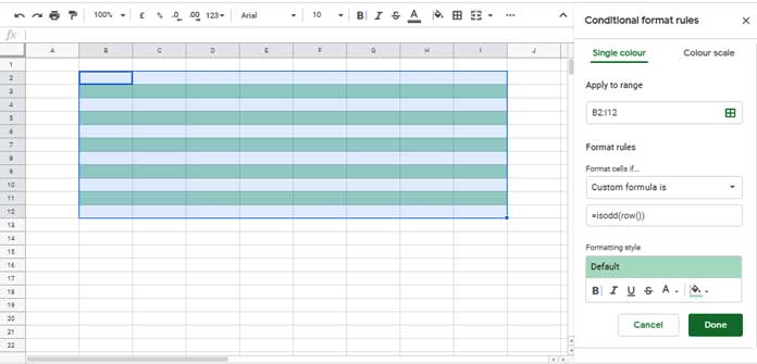

ISODD function used in conditional formatting rule

Tip: For basic alternating row colors, you can also use the built-in option under Format > Alternating colors. Use the ISODD formula when you need more customized or dynamic formatting.

Highlight Every Other Column:

=ISODD(COLUMN())

ISODD in Filtering

Filter only odd-numbered rows or columns.

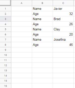
Filter Odd Rows:

=FILTER(
   B1:B8, 
   ISODD(
      SEQUENCE(ROWS(B1:B8))
   )
)

Filtering every alternate odd row in Google Sheets

Filter Odd Columns:

=FILTER(
   B1:H1, 
   ISODD(
      SEQUENCE(1, COLUMNS(B1:H1))
   )
)

Error Notes and Behavior

If the input is text, ISODD returns a #VALUE! error.
Decimal values are truncated to integers.

=ISODD(2.9)   → Same as ISODD(2) → FALSE

Zero (0) is considered even: =ISODD(0) returns FALSE, and so do empty cells.

Summary: When to Use the ISODD Function

Use the ISODD function in Google Sheets when you need to:

Check if a number is odd
Alternate row or column formatting
Create logical rules in IF statements
Filter odd-indexed data in structured ranges