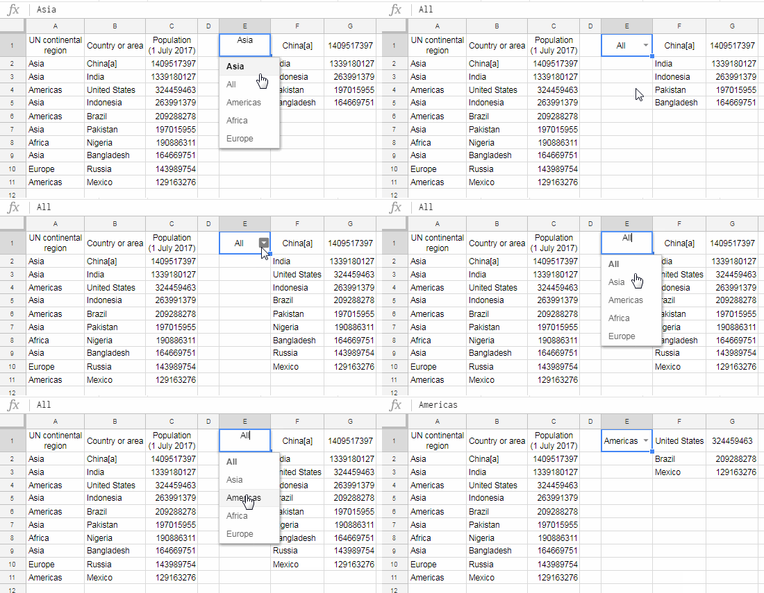
What about getting an “All” or “Any” selection option in a drop-down menu to populate part or whole data in Google Sheets?
I was about to write a tutorial on using drop-down menus in Charts. Along the way, I came across one issue. I wanted to visualize my data as a whole or in parts by applying different filters. I badly needed the option to select all the data from a custom drop-down menu.
This means I wanted a drop-down menu item called “All” or “Any” along with other categories (menu items) to filter my data for the chart.

How to Get an “All” or “Any” Selection Option in a Drop-down
Data Validation lets users create drop-down menus. You can insert it from the menu: Insert > Drop-down or Data > Data validation in Google Sheets.
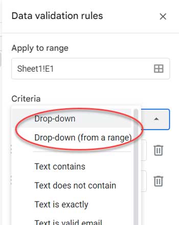
In a drop-down menu, you can add menu items in two ways:
- Drop-down
- Drop-down (from a range)

If you choose the “Drop-down” criteria, you need to add the menu items manually. This allows you to include an “All” menu item directly.
On the other hand, if you choose “Drop-down (from a range)” as the criteria, you select a cell range to include as the menu items.
However, there won’t be an “All” option in the drop-down unless the range already contains that value.
How Do We Add an “All” Option When Using Drop-down (from a Range)?
If your range is A2:A, you can create a new range with an “All” option by inserting the following formula in an empty column:
={"All";UNIQUE(A2:A)}Note: As per the sample data in the GIF above, I placed this formula in cell J2. The drop-down in cell E1 then uses the range J2:J instead of A2:A.
I hope you’ve learned how to include an “All” selection option in a drop-down menu in Google Sheets. Now, let me explain how to use this menu to filter your data using either the FILTER or QUERY functions.
Applying a Filter Based on the “All” Selection
Google Sheets offers a Filter menu option and a FILTER function. You can use drop-down menu items as criteria in the FILTER function to retrieve part or all data from a range.
For example, in the GIF, I used a drop-down menu to filter the data on the left-hand side. When I select “All,” the filter returns the entire dataset.
In cell F1, I applied the following Filter formula:
=ArrayFormula(IF(E1="All", B2:C11, FILTER(B2:C11, A2:A11=E1)))Here’s how it works:
- If the drop-down selection is “All,” the formula executes the
TRUEpart of the IF function, returning the rangeB2:C11as it is. - Otherwise, it filters
B2:C11based on the drop-down selection, i.e.,A2:A11=E1.
Using the Query Alternative
Here’s how you can achieve the same result with a Query formula:
=QUERY(A2:C11, "Select B,C " & IF(E1="All",, "where A = '"&E1&"' "),0)Need Multiple Drop-downs with “All” Selection?
If you need multiple drop-down menus with an “All” selection option for filtering multiple categories, check out:
Select All or a Specific Category in Multiple Columns in Filter in Google Sheets


Hi Prashanth,
This is a really useful article – many thanks for sharing. I’m using the formula provided with great success but now I’m stumped – I’d also like to filter my data using a second and possibly third drop down but I can’t figure out how to apply the ‘filter all’ element of the if statement to the second and/or third drop-down menus.
So a ‘customer name’ is selected from the first drop-down menu I’d like to see all the records relating to that customer, but then I’d like to filter the returned data using the second drop down to display all or filter by ‘subject’ and finally I’d like to filter the resulting data by all or ‘status’.
I feel like I’m stretching my capabilities here – is it even possible?
Gus
Hi, Gus,
Here is a link to my Sheet which contains a two-level All Selection.
Data Validation Eg
Best,
Hello,
Thank you for these amazing tips. It is helping me a lot. I have a question now, how will look like the formula when using 2 or more drop-downs?
=ArrayFormula(if(E1="All",B2:C11, filter(B2:C11,A2:A11=E1)))Hi, Josef,
I am glad that you liked this tutorial. Now answer to your question.
In my above example, there is only one drop-down, that is in cell E1. With that, you can only select all the countries or countries in any ONE continent. You can change that to all the countries or countries in any TWO continents.
To do that add one more drop-down in cell E2. You can just copy the drop-down in cell E1 and paste it in cell E2.
Now you can use this formula in cell F1.
=ArrayFormula(if(E1="All",B2:C11, filter(B2:C11,(A2:A11=E1)+(A2:A11=E2))))This formula reveals how to use the OR criteria in Filter. To learn more about this usage, please check my following related tutorial – How to Use AND,OR with Google Sheets Filter Function – ADVANCED Use.