


")


")

")
")
 in Excel & Google Sheets")


Highlighting the max value in each group in Google Sheets can make your data easier to read, more insightful, and visually compelling—especially when you’re analyzing grouped data like sales by region, student scores by class, or expenses by category.
While it’s straightforward to highlight the highest value in a range using the MAX function, doing it within each group (like one row per region or product line) isn’t as obvious. In these cases, MAX alone won’t cut it.
Tip: If you simply want to highlight the highest value in a single range, you can use a custom formula like =B2=MAX($B$2:$B). Just replace B2 with the top cell in your apply-to range, and adjust $B$2:$B to your actual column range.
In this tutorial, let’s walk through how to highlight the max value category-wise in Google Sheets, why it’s useful, and how to apply it using a custom formula with conditional formatting.
Why Highlight the Max Value in Each Group?
When your data is grouped—say by region, category, or department—it’s often helpful to quickly spot the top-performing item in each group. Instead of scanning rows and comparing values manually, the highlighted max values stand out instantly, making patterns easier to spot and decisions faster to make.
Some practical examples:
- Sales dashboards: Highlight the highest-selling rep in each region.
- Education data: Call out the top scorer in each class or subject.
- Budget reports: Identify the biggest expense within each category.
- Survey results: Show the most-liked aspect for each product or service.
Any time you want to visually pick out the “best” in each group, this approach does the trick.
Sample Dataset
Let’s use this simple dataset of sales reps and their numbers by region. It’s already sorted by region, though sorting isn’t required—the rule works either way.
| Region | Rep | Sales |
|---|---|---|
| Delhi | Alex | 3200 |
| Delhi | Divya | 4100 |
| Delhi | Mukul | 3900 |
| Mumbai | Dana | 2800 |
| Mumbai | Sam | 4600 |
| Mumbai | Roy | 4200 |
| Kochi | Ravi | 3100 |
| Kochi | Kajol | 3300 |
| Kochi | Omar | 3300 |
The goal is to highlight the max value in each group—in this case:
- 4100 in Delhi
- 4600 in Mumbai
- 3300 in Kochi (shared by two people)
Custom Formula to Highlight the Max Value in Each Group
To create the rule, we’ll use two columns:
- Region – the group column (Column A)
- Sales – the value we’re checking for maximum (Column C)
Formula Using MAXIFS
=AND(C2<>"", C2=MAXIFS($C$2:$C, $A$2:$A, A2))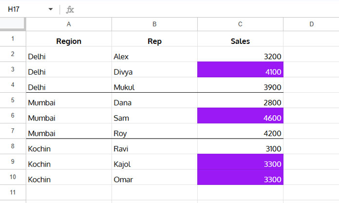
How it works:
MAXIFS($C$2:$C, $A$2:$A, A2)returns the highest Sales value for the current Region.C2=...checks if the current Sales value is that max.C2<>""ensures we skip blank rows (optional but useful).- If all conditions are true, the cell is highlighted.
Related: MAXIFS Function in Google Sheets: Find Maximum Value Conditionally
Alternate formula using FILTER
=AND(C2<>"", C2=MAX(FILTER($C$2:$C, $A$2:$A=A2)))This version:
- Filters the Sales values for the current Region using FILTER.
- Finds the max from those filtered values.
- Compares it to the current row’s Sales.
Both formulas work the same way in practice—pick the one you’re more comfortable with.
How to Apply the Rule
Here’s how to highlight the max value in each group using conditional formatting:
- Select the Sales column, starting from the top cell you want to highlight. For our dataset, select
C2:C10(or as far down as your data goes). - Go to Format > Conditional formatting.
- Under Format cells if, choose Custom formula is.
- Paste the formula:
=AND(C2<>"", C2=MAXIFS($C$2:$C, $A$2:$A, A2)) - Choose a fill color to highlight the max value.
- Click Done.
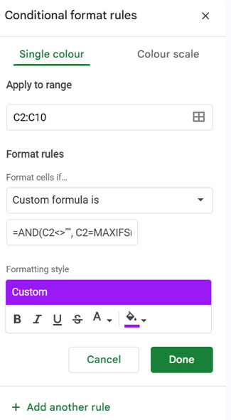
Make sure the “Apply to range” starts from the same row as in your formula (C2 in this case). The formula will evaluate each row and apply formatting to cells that meet the condition.
Resources
- How to Highlight Groups That Exceed a Target in Google Sheets
- Highlighting Multiple Groups and Control Tick Boxes in Google Sheets
- How to Highlight the Min Value in Each Group in Google Sheets
- Conditional Formatting Based on Data Groups in Google Sheets
- Alternating Colors for Groups and Filtering Issues in Google Sheets
- Highlight Groups with Alternating Colors in Excel
Can you use this same technique to find the minimum in each group?
Hi, Randall Revere,
It’s so simple. Please check my new tutorial – How to Highlight the Min Value in Each Group in Google Sheets.
PERFECT!!! Thank you
Hi, Randall Revere,
I’ve modified the post. You can find a much simpler Rule # 2 there now.
Copy that instead.
=B1=MAX(FILTER(B:B, A:A=A1))Where;
A is the category column.
B is the value column.
Hi, Dev L,
This is cool! Thanks for sharing.