")
")


")


")

")
")
 in Excel & Google Sheets")


A floating column chart in Google Sheets is a visual tool that shows the range between two values—such as minimum and maximum temperatures or the high and low prices of a stock—by using a modified stacked column chart. It resembles a candlestick chart but only highlights the low and high values, making it ideal for scenarios where open and close values are not required.
In this tutorial, you’ll learn how to create a floating column chart in Google Sheets using simple formulas and chart settings.
What Is a Floating Column Chart?
A floating column chart (also known as a high-low chart or floating bar chart) displays a vertical bar that “floats” between a minimum and a maximum value. Since Google Sheets doesn’t offer this chart type directly, we simulate it by:
- Using a stacked column chart, and
- Making the bottom (minimum) value series transparent.
When to Use a Floating Column Chart
You can use this chart to visualize:
- Minimum and maximum temperature over time
- Low and high prices of a stock
- Any two numerical values representing a measurable range (e.g., budgeted vs. actual cost)
Example 1: Temperature High and Low Values for a Week
Step 1: Prepare Your Data
Paste the following data in A1:C8:
| Date | Min Temp (°C) | Max Temp (°C) |
| 20/05/2019 | 27 | 32 |
| 21/05/2019 | 27 | 33 |
| 22/05/2019 | 27 | 33 |
| 23/05/2019 | 27 | 33 |
| 24/05/2019 | 27 | 32 |
| 25/05/2019 | 27 | 32 |
| 26/05/2019 | 27 | 32 |
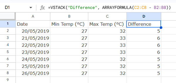
Step 2: Calculate the Difference
In cell D1, enter this formula:
=VSTACK("Difference", ARRAYFORMULA(C2:C8 - B2:B8))This gives you the range between Min and Max temperatures.
Step 3: Create the Chart
- Select the range A1:D8
- Go to Insert > Chart
- In the Chart Editor:
- Set Chart type to Stacked Column Chart
- Remove the Max Temp series under Setup > Series
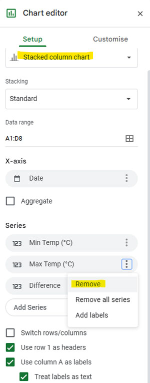
- Go to Customize > Series
- Select the Min Temp series
- Set the color to white or transparent by setting the Opacity to 0%
- (Optional) Go to Customize > Legend and set the Position to None to remove the legend
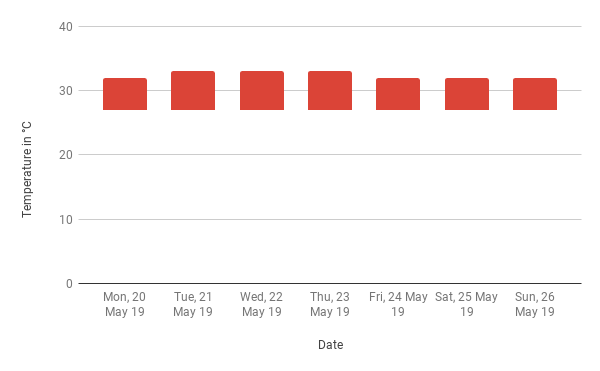
The result is a clean floating column chart where the columns represent only the temperature range.
Example 2: Stock Price Range Using GOOGLEFINANCE
Step 1: Import Low and High Prices
In cell A1, use the GOOGLEFINANCE function to pull low and high prices for a stock:
=LET(
   gfData,
   GOOGLEFINANCE("GOOG", "All", DATE(2025, 4, 1), DATE(2025, 4, 30)),
   CHOOSECOLS(gfDATA, 1, 4, 3)
)
Step 2: Calculate the Difference
In cell D1, enter:
=VSTACK("Difference", ARRAYFORMULA(IF(LEN(A2:A), C2:C - B2:B, )))Step 3: Insert the Chart
- Select A1:D
- Go to Insert > Chart and set it to Stacked Column Chart
- Remove the High series under Series
- In Customize > Series, select the Low series and set the color to white or transparent
- (Optional) Go to Customize > Legend and set Position to None
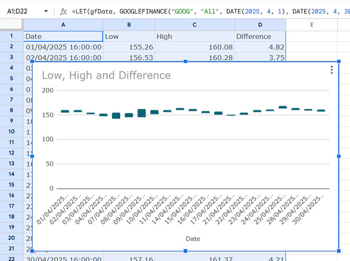
You now have a floating chart showing the daily range of stock prices.
Floating Column Chart vs. Candlestick Chart
| Chart Type | Shows | Best For |
|---|---|---|
| Floating Column Chart | Min & Max only | Temperature, price ranges |
| Candlestick Chart | Open/High/Low/Close | Detailed stock trading analysis |
If you only need high and low values, floating column charts are simpler and cleaner.
FAQs
Q: Can I make a high-low chart in Google Sheets?
Yes! Google Sheets doesn’t have a built-in option, but a stacked column chart with the base hidden can simulate it.
Q: What’s the difference between a floating column chart and a candlestick chart?
Candlestick charts show open, high, low, and close values. Floating column charts show only the range between low and high.
Q: Can I use floating charts for non-financial data?
Absolutely. They’re great for temperature, time tracking, or any other high-low value visualization.